15. Two-Slit Interference: Young’s Experiment

15.1. Historical context

There is a rich historical background behind the experiment you are about to perform. Isaac Newton first separated white light into its colors, and in the 1680’s hypothesized that light was composed of ‘corpuscles’, supposed to possess some properties of particles. This view reigned until the 1800’s, when Thomas Young first performed the two-slit experiment now known by his name. In this experiment he discovered a property of destructive interference, which seemed impossible to explain in terms of corpuscles, but is very naturally explained in terms of waves. His experiment not only suggested that such ‘light waves’ existed; it also provided a result that could be used to determine the wavelength of light, measured in familiar units. Light waves became even more acceptable with dynamical theories of light, such as Fresnel’s and Maxwell’s, in the 19th century, until it seemed that the wave theory of light was incontrovertible. And yet the discovery of the photoelectric effect, and its explanation in terms of light quanta by Einstein, threw the matter into dispute again. The explanations of blackbody radiation, of the photoelectric effect, and of the Compton effect seemed to point to the existence of ‘photons’, quanta of light that possessed definite and indivisible amounts of energy and momentum; These are very satisfactory explanations so far as they go, but they throw into question the destructive-interference explanation of Young’s experiment. Does light have a dual nature, of waves and of particles? And if experiments force us to suppose that it does, how does the light know when to behave according to each of its natures? These are the sorts of questions that lend a somewhat mystical air to the concept of duality. Of course the deeper worry is that the properties of light might be not merely mysterious, but in some sense self-contradictory.

It is the purpose of this experimental apparatus to make the phenomenon of light interference as concrete as possible.

Here, then, are the goals of the experiments that this apparatus makes possible:

1. You will be seeing two-slit interference visually, by opening up the apparatus and seeing the exact arrangements of light sources and apertures which operate to produce an ‘interference pattern’. You’ll be able to examine every part of the apparatus, and make all the measurements you will need for theoretical modeling.

2. You will be able to perform the two-slit experiment quantitatively, recreating not only Young’s measurement of the wavelength of light, but also getting detailed information about intensities in a two-slit interference pattern which can be compared to predictions of wave theory of light.

3. You will be exploring a theoretical model which attempts to describe your experimental findings. You will thus encounter Fraunhofer diffraction theory in a concrete case.

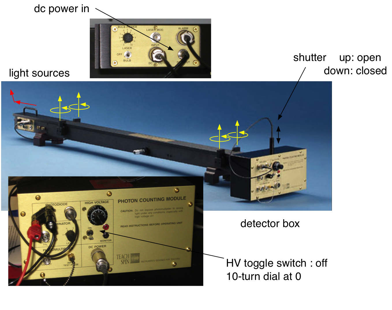
Fig. 15.1 Overview of the two-slit interference apparatus.

15.2. Experimental Setup

The apparatus is shown in Fig. 15.1 . Orient it on its wooden feet so that the detector box is at the right hand end of the assembly, and you’ll be properly oriented to match the parts of the apparatus with the description below. First (before plugging anything in, or turning anything on ) you’ll need to make sure that the shutter, which protects the amazingly sensitive single-photon detector, is closed (pushed all the way down, take this opportunity to try pulling it vertically upward by about 2 cm, but then ensure that it’s returned to its fully down position). Confirm, on the detector box, that the toggle switch in the HIGH-VOLTAGE section is turned off and that the 10-turn dial near it is set to 0.00, fully counter-clockwise.

Now it’s safe for you to open the cover of the long two-slit assembly. Before you can do this, you’ll need to open the four latches that hold it closed; execute a slight lift and a quarter-turn of each of these latches until they are visibly disengaged (yellow arrows). The cover is still light tight and rather snugly closed, so you may want to lift it off by screwing in the brass thumbscrew at the far-left end of the cover. Then lift (by a cm or more) the far-left end of the cover of the apparatus. Now slide the whole cover sideways and leftwards by a cm or more (red arrows); this will disengage the right end of the cover from its light-tight slot, so you can lift the whole cover off. ( Take this opportunity to learn how to re-install the cover, making sure that you can engage its right end, lower its left end, back off the thumbscrew, and reengage the four latches which hold it in place. ) With the cover open, you are ready to look over all the parts of the apparatus as shown schematically in Fig. 15.2.

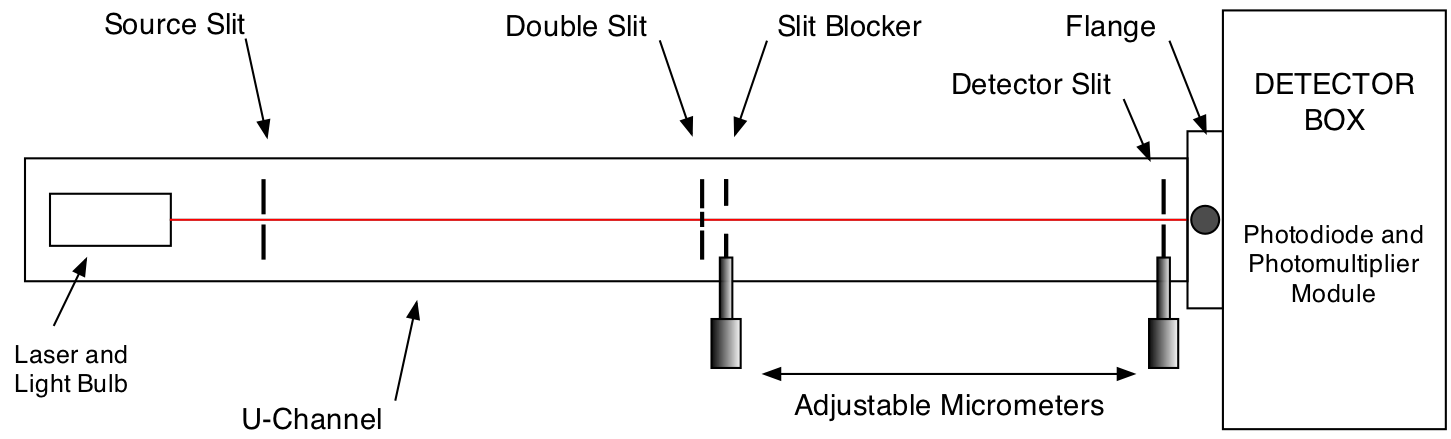
Fig. 15.2 Schematic of the arrangement of light sources, slits and detector.

The two micrometer drives on the front allow you adjust the horizontal position of the slit blocker and the detector slit. There are two distinct light detectors in the detector box:

1. One is called a ‘photodiode’, which is used with the much brighter laser light source; it’s attached to the light shutter in such a way that it’s in position to use when the shutter is in its down position.

2. The other is called a ‘photomultiplier tube’ or PMT for short, which is used with the much dimmer light-bulb source for single photon counting. It will not be used in this experiment. It is safe to use only when the cover of the apparatus is in place, and the light bulb is in use; it is exposed to light only when the shutter is in its up position.

Finally, there are electrical connections. Electric power comes from a power module, plugged into your AC-line and connected by a cable to the left end of the apparatus (Fig. 15.1). Two more cables run from this end to the detector box, and supply the photodiode and PMT detectors with the power they need for operation (have your instructor check all connections).

15.3. Optical Alignment

Before you take on the task of aligning the apparatus, it is worth examining all the slits. Each slit is stamped in a metal foil, whose edge is attached to a magnetic fixture that allows it to be placed conveniently in a slit-holder in the apparatus. Practice taking the source slit right off of its holder, and look it over with a magnifying glass. You’re looking at a single slit, and you’ll want to know its width; this can be measured by single- slit diffraction or using the traveling microscope.

In the same way you can also characterize the detector slit, and the wide slit whose two edges are used to execute the slit-blocking functions. Finally, examine one or more of the double-slit assemblies that are available; for these you will want not only to measure the width of the two individual slits, but also to determine their separation. However you measure this separation, it is conventional to characterize a double slit by the center-to-center separation of the two slits. As you replace the slits, you’ll note that they can be translated both vertically and horizontally to a limited extent; it is also possible to rotate them to some extent in their own plane. For best results, you want all the slits to have their long edges set to be accurately vertical; for the moment, use an ‘eyeball accuracy’ criterion for this.

Now it’s time to align the whole apparatus

1. Ensure that the PMT shutter is closed, and the PMT bias is turned off (by toggle switch) and down (to 0.00 on the 10-tum dial). Now connect the line cord to AC power, and turn on the laser source - use a paper card to see the beam.

2. Align the laser beam and the slits in the apparatus (this should not always be necessary):

   • Put the detector slit in first, and do your best to make the slit’s edges vertical.

   • Put in the slit-blocker (the wide slit), and use a card just downstream of it to see the broad stripe of light that it permits to pass through.

   • Put in the double slit, and now find the two narrow vertical ribbons of light that come through it. (Adjust the slit-blocker, using its micrometer, to ensure that both ribbons will pass through to your card.)

   • Put in the source slit. This will at first block the laser beam, so adjust the slit (not the laser) by lateral translation in its plane, until it is centered on the beam.

   • To do the final adjustment of the source slit’s position, look at the upstream side of the double-slit fixture, and find the single-slit diffraction pattern projected there by light passing through the source slit. Do a by-hand fine-adjust of the source slit’s location, until the central maximum of this single-slit diffraction pattern is centered on the double-slit structure. You can confirm that you’ve done this optimally by placing a viewing card downstream of the double slits and slit-blocker, and checking that the source slit has been moved so as to maximize the brightness of The laser light emerging from the double slits in two bright vertical ribbons of light.

   • Alignment of the slit-blocker: your goal is to get its two long edges aligned to be vertical. You may start by removing the slit-blocker’s (wide) slit from its magnetic mount; remember the slit-blocker is mounted on the micrometer-adjusted, flexure-supported moveable block just downstream of the double slits. The best diagnostic for the proper positioning of the slit-blocker’s wide slit is to use the two ribbons of light emerging beyond the double slit when they are illuminated ‘by the laser source. Find these ribbons on a paper card, and now re-install the wide slit on its mount. Use the micrometer to translate the wide slit laterally until both ribbons emerge, and now dial the micrometer until you see the knife-edge function of the slit-blocker in cutting off one of the ribbons of light. If the wide slit is in place with its edges not correctly vertical, this knife-edging of the ribbon will proceed not all at once, but bottom-to-top or top-to bottom. Hand-adjust the wide slit by small in-plane rotations on its magnetic holder until you achieve the desired all-at-once chopping-off of the ribbon of light.

   • The equivalent alignment task for the detector slit is to rotate it in its own plane, until its length is accurately parallel to the double-slit fringes that it is to scan. The best diagnostic for this is the contrast of the interference pattern that you will record later. So for now, just be sure that the detector slit is vertical to eyeball accuracy.

3. The instrument should now be aligned and ready for measurements.

At the detector end of the apparatus, you’ll need a digital multimeter for reading the output voltage that emerges from the photodiode-amplifier mode of detection. You can understand this signal by noting that the photodiode translates input optical power to output electrical current with a sensitivity of about 0.4 A/W (Exercise: show that the conversion of photons of red light to electron-hole pairs in a semiconductor with 100% efficiency would yield about 0.5 A of output current for an input of l Watt of optical power.), and then the photodiode amplifier translates photodiode current to output voltage with a conversion constant of \(22\cdot 10^6\) V/A. So if we see an output of 1.0 Volt, we can infer an input current of \(4.5 \cdot 10^{-8} A = 0.045 \mu A\), and further infer an incident optical power of \(11 \cdot 10^{-8} W = 0.11 \mu W\), on the photodiode. The photodiode amplifier has a time constant of \(0.4 ms\), which sets the timescale for the response time of this detector system.

Also at the detector end of the system are the electronics for running the photomultiplier tube which we will not need here so DO NOT TOUCH IT.

15.4. Measurements

15.4.1. Visual Exploration

You will be working first with the cover of the apparatus open. Use the controls at the left end to turn on the solid-state diode-laser light source. Use a paper screen to find its bright red output beam; the diode laser manufacturer asserts that its output wavelength is \(670 \pm 5 nm\) and its output power is about 5 mW. (So long as you don’t allow the full beam to fall directly into your eye, it presents no safety hazard) Follow the laser beam until it reaches the entrance slit, or source slit, of the two-slit apparatus; this is a single slit, of height about 1 cm, but width of only 0.085 mm. If your apparatus is aligned, the slit will be neatly straddling the laser beam, so that a good fraction of the laser light will be passing through the slit - use your paper card to see if this is so. Light passing through this narrow source slit will undergo ‘single-slit diffraction’, and you can follow this process by moving your viewing card downstream. In the middle of the apparatus is the holder for the double slit. Put your viewing card just downstream of the two-slit structure, and look (close up) to see if you can observe the two ribbons of light, just a fraction of a millimeter apart, which emerge from the two slits.

You have three distinct two-slit assemblies; if you look at one of your spares, you’ll see a number (14, 16, or 18) hand-written onto the metal film into which the double slits are stamped. This number is the nominal center-to-center separation of The two slits, given in units of ‘mils’ = 0.001” \(= 25.4 \mu m\). So the slit separations available to you are nominally 0.356 mm, 0.406 mm, and 0.457 mm.

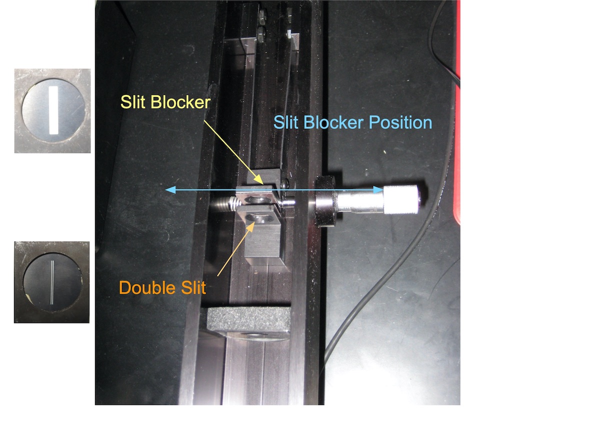
Fig. 15.3 The slit blocker used to select the slits (left, both, right)

A micrometer screw will move the slit-blocker ( a wide slit, Fig. 15.3) laterally across the two ribbons of light emerging from the two-slit system. Find a position for the micrometer adjustment that permits the two ribbons of light to emerge and continue rightwards in the apparatus. Follow with your card to the location of the detector slit. Position a viewing card at the downstream end so you can refer to it for a view of the fringes, and take another card back upstream to the vicinity of the slit-blocker. Start by rotating the multi-turn micrometer fully clockwise, and watch this adjustment push the slit-blocker away from you.

Find and record three key settings for the slit-blocker’s micrometer:

1. One for which light emerges only from the right one of the two slits when looking toward the detector.

2. One (anywhere in a wide range) that allows both ribbons of light to emerge

3. One for which light emerges only from the left one of the two slits

Check with your viewing card at the detector slit position for each of the 3 positions. Describe what you observe.

15.4.2. Measurement of the Intensity Distribution

You will measure the intensity distribution of the interference pattern using the photo diode. Close up the cover of the apparatus. Set the slit-blocker to that previously determined setting which allows light from both slits to emerge and interfere. The shutter of the detector box must be in its closed, or down, position. This blocks any light from reaching the PMT, but the shutter in its down position correctly centers a \(1 cm^2\) solid-state ‘photodiode’, which acts just like a solar cell in actively generating electric current when it’s illuminated. The detector slit (Fig. 15.4) makes sure that the only light reaching the detector is that from a selected part of the interference pattern; by this means, a single- element, spatially-fixed, large-area detector can serve to record (serially in time) the intensities at various places in the interference pattern.

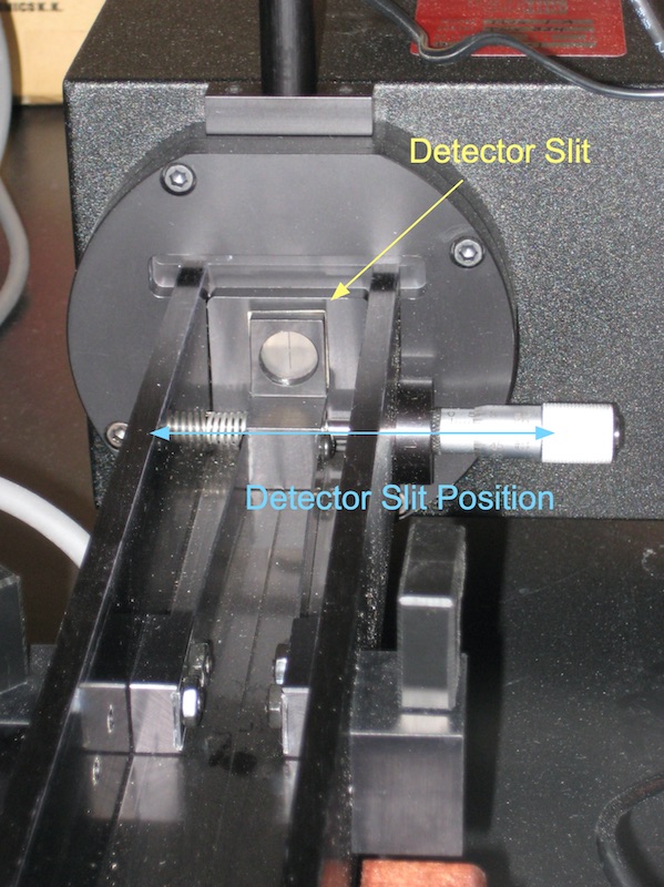
Fig. 15.4 Detector slit with moving mechanism and micrometer.

The method of course relies on the fact that the rest of the apparatus is stable in time; the diode-laser source has an output power varying by <0.l% in time, and the mechanical stability of the rest of the apparatus is also adequate.

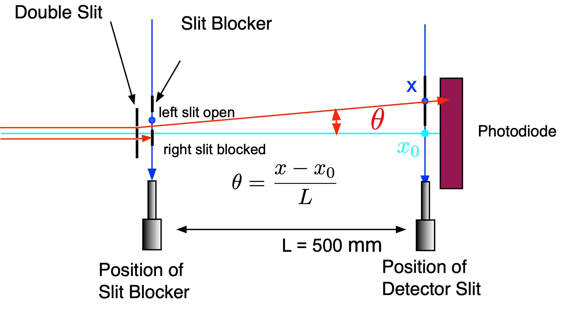
Fig. 15.5 Geometry of double slit, slit blocker, detector slit and detector.

15.5. Photodiode Checkout

The electric current from the photodiode is conducted by a thin coaxial cable to the INPUT BNC connector of the photodiode-amplifier section of the detector box. At the OUTPUT BNC connector adjacent to it, there appears a voltage signal derived from that photocurrent.

1. Connect to this output a digital multimeter set to 2 or 20-Volt sensitivity; you should see a stable positive reading.

2. To determine if this reading means anything, turn the laser source off. This should reduce the voltage signal but perhaps not to zero; record the value you see, and take it to be the ‘zero offset’ of the photodiode-detector system. The zero-offset reading will eventually need to be subtracted from all the other readings you make of this output voltage.

3. Turn your laser source back on, and now watch the photodiode’s voltage-output signal as you vary the setting of the detector-slit micrometer.

4. If all is well, you will see a systematic variation of the signal as you dial the micrometer; you are scanning over the interference pattern. Measure the patterns in small enough steps that you can determine minima and maxima locations and intensities.

5. Between the various maxima, you should see minima; and if your alignment is good, the signal at these minima should drop nearly to the zero-offset signal, if the variation is only slightly then your alignment needs to be improved.

15.6. Pre-Lab Preparation

1. The experiment is called double-slit. However, one should also be able to observe interference patterns even if there is only a single slit for the laser light to pass through. Why? Use your own words.

2. Prepare the data file (header etc.) to enter the measured data

3. Prepare a small python script to plot the data while you are taking them

4. Bonus: what would be the expression for the intensity for a double slit where the slit widths are not equal?

15.7. Analysis

1. Convert the micrometer readings to viewing angles (you need to determine the distance between the double slit and the detector slit see Fig. 15.5 ).

2. Plot the observed intensity (the voltmeter reading) as a function of angle.

3. Normalize your data in such a way that the highest intensity is one. The angle with the highest intensity corresponds usually to \(\theta = 0.\)

4. Determine each single slit width by fitting the normalized single slit interference pattern with function (15.2) with \(A_0, D, x_0\) as parameters

5. Determine the slit separation S and the common slit width D of the double slit by fitting the normalized double slit interference pattern with function (15.3) and \(A_0, S, D, x_0`\) as fit parameters.

6. Measure the double slit geometry by using the traveling microscope and determine \(D, S\) include their errors.

7. Compare and discuss the different results.

15.8. Single and Double Slit Interference Patterns

The intensity distributions can be understood using Fraunhofer diffraction (assuming source and observation point are at infinity). Fig. 15.6 shows the construction of the total amplitude for a single slit. The slit is divided into identical small \(dx\) wide strips. Each strip contributes an amplitude \(d\vec{A_0}\) represented by a vector (phasor). The contribution of each strip experiences a path length difference of \(\Delta\) with respect to the previous one resulting in a phase shift \(d\delta = (2\pi/\lambda) \Delta\).

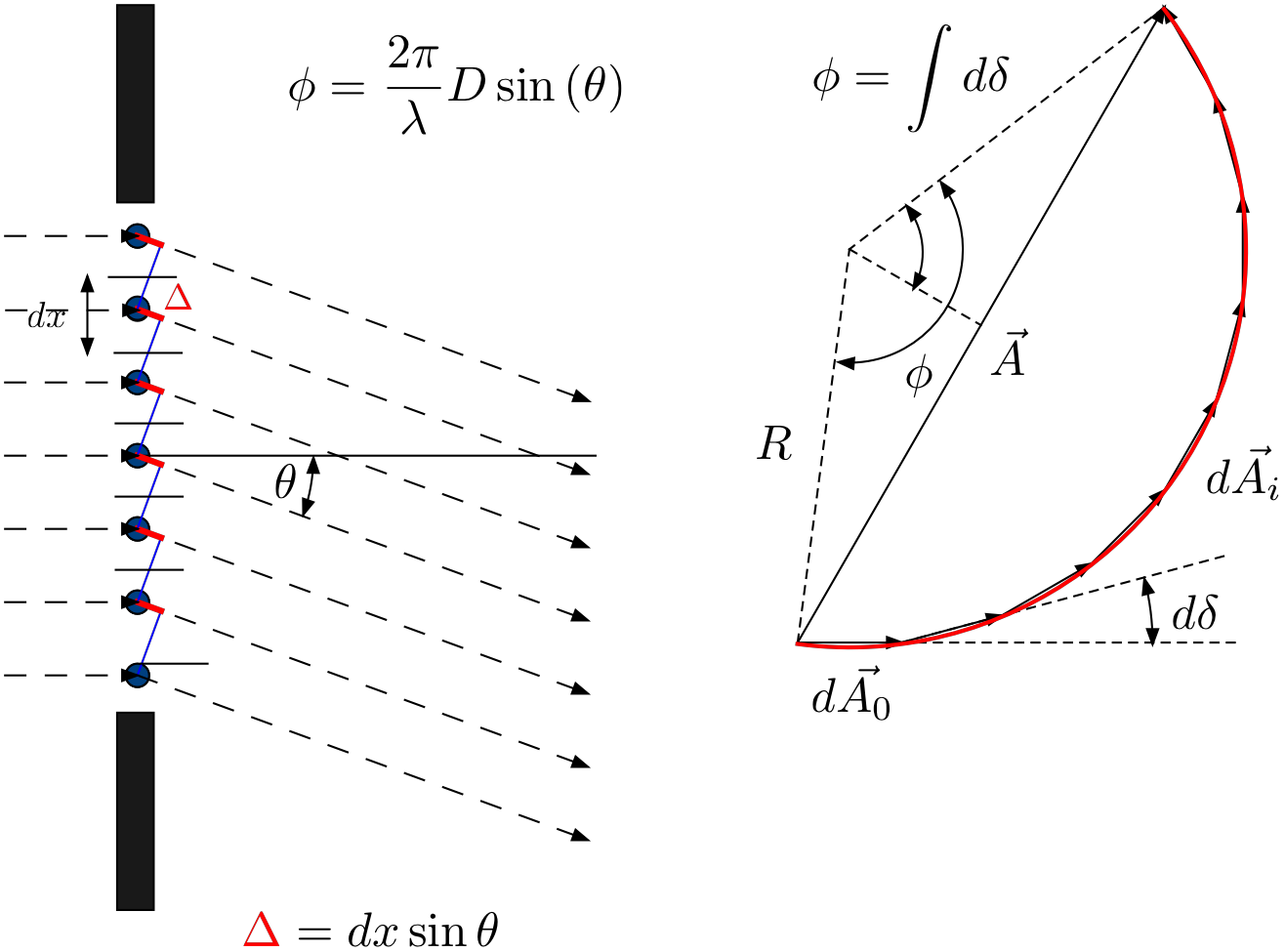
Fig. 15.6 Phasor diagram for calculating the total amplitude for Fraunhofer diffraction from a single long slit.

For the total amplitude one obtains:

(15.1)\[ \begin{align}\begin{aligned}\vec{A} = \sum_i^N{d\vec{A_i}}\\|d\vec{A_i}| = \frac{dx}{D}|\vec{A_0}|\end{aligned}\end{align} \]

If \(N\rightarrow \infty\) one obtains for the final amplitude \(|\vec{A}| = 2 R \sin{(\phi/2)}\) with \(\phi = \frac{2\pi}{\lambda}D\sin{(\theta)}\) and \(R = |\vec{A_0}|/\phi\). Putting everything together:

(15.2)\[ \begin{align}\begin{aligned}|\vec{A}| = |\vec{A_0}|\frac{\sin{(\phi/2)} }{\phi/2.}\\I(\theta) = I_0 \left( \frac{\sin{(\phi/2)} }{\phi/2.} \right)^2\end{aligned}\end{align} \]

Where \(I(\theta)\) is the intensity observed at an angle \(\theta\).

Combining two identical slits a distance \(S\) appart as shown in Fig. 15.7.

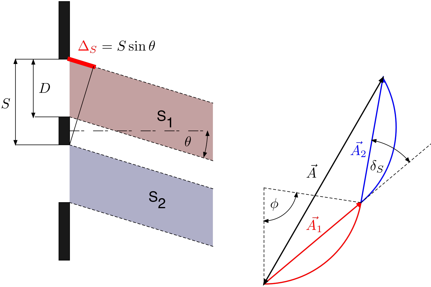
Fig. 15.7 Combining the total amplitude of two identical slits to the combined amplitude describing double slit interference.

one needs to include an additional phase shift \(\delta_S = k S\sin{(\theta)}\) due to the separation of the slits. Each of the amplitudes \(\vec{A_1}\) and \(\vec{A_2}\) have the same magnitude and one obtains for the final result:

(15.3)\[ \begin{align}\begin{aligned}|\vec{A}| = | \vec{A_1} + \vec{A_2} | = 2|\vec{A_0}|\frac{\sin{(\phi/2)}}{\phi/2}\cos{(\psi/2)}\\I(\theta) = |\vec{A}|^2\end{aligned}\end{align} \]

where \(k = 2\pi/\lambda\), \(\phi = kD\sin{(\theta)}\) and \(\psi = kS\sin{(\theta)}\). Note: you measure the intensity \(I(\theta)\) NOT the amplitude.

15.9. Programming Hints:

Here is an example on how to fit the double slit interference pattern ((15.3)). It will use the a general non-linear fit (Look at the documentation general non-linear fitting) since the intensity distribution is not a linear function of all fit parameters:

Here are some steps how to setup the fit function:

D = B.Parameter(1.e-4, 'D')  # slit width in m, initial value set to 0.1mm
S = B.Parameter(3.e-4, 'S')  # slit separation in m, initial value set to 0.3mm
x0 = B.Parameter(1.e-2, 'x0') # location of maximum in position, initial value set to 0.01 radian, you need to adjust this to your data
I0 = B.Parameter(1., 'I0') # Max. intensity, initial value set to 1

With these parameters you can now define your fitting function as follows (this is one of many possibilities, check that it agrees with eq. (15.3) ):

def Intensity(x):
    k = 2.*np.pi/lam                # lam is the wavelength
    phi = k*D()*np.sin((x-x0())/L)  # L is the distance between the double slit and the detector slit
    psi = k*S()*np.sin((x-x0())/L)
    I = I0()*(np.sin(phi/2.)/(phi/2.))**2 * np.cos(psi/2.)**2
    return I

You should now try to calculate an angular distribution and plot it to compare the curve to your data. To do this do the following, I assume \(\theta_{min},\theta_{max}\) are the two limiting angles (in radians) corresponding to the extreme positions of your detector slit:

th = np.linspace(tmin,tmax, 1000) # create an array of 1000 equally spaced values between tmin and tmax
D.set(0.8e-4)  # change the value of D to 0.08 mm
S.set(3.1e-4)  # change the value of S to 0.31 mm
B.plot_line(th, Intensity(th))  # this should plot the calculated line with the new parameter values

See how the curve changes and play with the parameters. Once you have found a set that looks somewhat similar to your data your can do the fit by doing:

i_fit = B.genfit(Intensity, [D,S,x0,I0], x=th_exp, y = I_exp, y_err = dI_exp) # assuming th_exp, I_exp, dI_exp
                                                                              # are your exp. data
B.plot_exp(th_exp, I_exp, dI_exp)
B.plot_line(i_fit.xpl, i_fit.ypl)  # this plots the fitted values

You should now have a nice fit of your measured intensity distribution. Look at the fitted parameters:

print D
print S
print I0
print x0

This will print their values and errors. Use the traveling microscope and measure the size of the double slit. Compare to your fitted values.

Setup a similar fit for the single slit interference pattern (equation (15.2)).