Data Fitting

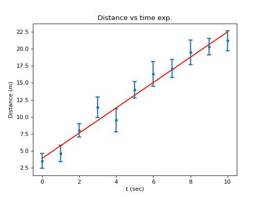
Very frequently one wants to try to extract an interesting quantity from the experimental data. I assume you know the functional relation ship between the different quantities but you do not know the parameters. As an example I take the example data: distance as a function of time. If the object was moving with constant velocity the distance should be a linear function of time, with the slope being the velocity and the y-axis offset the position at \(t = 0\). To do this I want to perform a least square fit of a line to the data.

Fitting a Line

In order to fit a line (\(y = ax + b\), where \(a\) is the slope and \(b\) is the y-axis offset) to your data you use the linefit function. This function needs the data as arrays, so I will use the array t for the time, dexp for the distance and derr for the errors in the distance. To carry out the fit do the following:

In [44]: fit = B.linefit(t, dexp, derr)

You should see the output

In [44]: fit = B.linefit(t, dexp, derr)
chisq/dof =  0.661037211585
offset  =  3.88359753039  +/-  0.540669925884
slope =  1.86063659417  +/-  0.098317559634

and a plot of the fitted line.

The fitted parameters can be accessed as follows:

\(a =\) fit.slope, \(b =\) fit.offset

And their uncertainties are:

\(\sigma_{a} =\) fit.sigma_s, \(\sigma_{b} =\) fit.sigma_o

Remember the slope is the velocity which in this case would be \(1.86\) with an uncertainty of \(\pm 0.1\) and and the position at \(t = 0\) is \(3.88 \pm 0.54\). The function returns much more information that you stored in the variable fit. To see it just enter fit.res and you will get:

In [45]: fit.res
Out[45]:
{'chisquare': 5.9493349042607102,
 'cov. matrix': array([[ 0.44222014, -0.06453747],
       [-0.06453747,  0.01462299]]),
 'deg. of freedom': 9,
 'difference': array([ 0.38359753,  1.14423412, -0.39512928, -1.93449269,  1.82614391,
       -0.8132195 , -1.2525829 , -0.19194631, -0.73130972,  0.32932688,
        1.28996347]),
 'fitted values': array([  3.88359753,   5.74423412,   7.60487072,   9.46550731,
        11.32614391,  13.1867805 ,  15.0474171 ,  16.90805369,
        18.76869028,  20.62932688,  22.48996347]),
 'parameters': array([ 3.88359753,  1.86063659]),
 'red. chisquare': 0.66103721158452333,
 'xpl': array([  0.,   5.,  10.]),
 'ypl': array([  3.88359753,  13.1867805 ,  22.48996347])}

fit.res is a Python dictionary, to see its keys only you can do:

In [46]: fit.res.keys()

and will get

In [46]: fit.res.keys()

Out[46]:
['red. chisquare',
 'parameters',
 'fitted values',
 'deg. of freedom',
 'xpl',
 'cov. matrix',
 'chisquare',
 'difference',
 'ypl']

To get the number of degrees of freedom in this fit, you would type

In [47]: fit.res['deg. of freedom']

And you would get back the number 9, try it ! A very important quantity is the covariance matrix for error propagation. It is also there and you can assign it to the variable named e.g. cov and display it by doing:

In [47]: cov = fit.cov
In [48]: cov

cov is a 2d array that can be used in error propagation later. It is also interesting to display the fitted line together with the data. First I draw the data using plot_exp() with the data arrays:

In [49]: B.pl.clf()
In [50]: B.plot_exp(t,dexp, derr); B.pl.show()

The fitted line is plotted automatically. It can also be drawn using the command below :

In [51]: fit.plot()

The linear fit is the one you will be mostly using in the analysis of your experiments. If you want to evaluate the fitted function (in this case a line) for any value \(x\). You use it as follows:

In [52]: y = fit(x)

y now contains the value of the fit function for the argument x

Here is the result with everything labelled:

(Source code)

Fitting a Polynomial

Maybe your data are not really for an object moving with constant velocity. If there is for instance an acceleration present the position would vary quadratically with time and the coefficient of the quadratic term would be proportional to the acceleration. You can try to determine this by fitting a polynomial of 2nd degree to the data using the function polyfit:

In this case the fit function would be:

\(f(x) = a_0 + a_1 x + a_2 x^2\)

and the corresponding python command:

In [53]: fitp=B.polyfit(t,dexp,derr,2)

You could also have done:

In [54]: fitp=B.polyfit(t,dexp,yerr=derr,order=2)

yerr and order are keyword arguments. The number 2 indicates the polynomial order. The result looks like:

In [43]: fitp=B.polyfit(t,dexp,derr,2)
chisq/dof =  0.519062589345
parameter [ 0 ] =  3.12859470397  +/-  0.627859702779
parameter [ 1 ] =  2.45054883094  +/-  0.3288132167
parameter [ 2 ] =  -0.061125765893  +/-  0.0328533890728

The corresponding parameters in this case are:

\(a_0 =\) fitp.par[0], \(a_1 =\) fitp.par[1], \(a_2 =\) fitp.par[2]

And their uncertainties are:

\(\sigma_{a_0} =\) fitp.sig_par[0], \(\sigma_{a_1} =\) fitp.sig_par[1], \(\sigma_{a_2} =\) fitp.sig_par[2]

As you can see there could be indeed a small negative acceleration. Also note that the complete fit results are stored in an object named fitp.res. You can plot the result of the quadratic fit by doing

In [55]: fitp.plot()

Which looks exactly like what you did for the line fit; all that has changed is the name of the result (here it is fitp before it was fit)

As for the case of the fitted line, the fitted polynomial can be used by:

In [56]: y = fitp(x)

y now contains the value of the fit function for the argument x.

In a general case, the function function polyfit fits a polynomial of order \(n\)

\(f(x) = a_0 + a_1 x + a_2 x^2 + ... + a_n x^n\)

The python command in this case would be:

In [57]: p=B.polyfit(x, y_exp,sigma_y,n)

The polyfit results are stored here in the variable p and the parameters \(a_i\) correspond to p.par[i] or the Parameter array p.parameters.

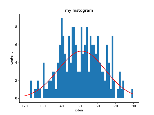
Histogram Fitting

Overview

The most frequently used fitting task in histograms is fitting a gaussian to a peak. This is useful to determine the location of a peak and other information on the peak shape such as width and height. Fitting a gaussian requires a non-linear fitting algorithm and is therefore a bit harder to use. The LT.box.histo object has a built-in fitting function that fits a gaussian on top of a quadratic background using the following fit function:

\(f(x) = b_0 + b_1x + b_2x^2 + A exp(-(x - \mu)^2/\sigma^2)\)

By default only the gaussian peak parameters, \(A, \mu, \sigma\), are fitted and the background parameters \(b_0, b_1, b_2\) are set to 0 and are kept constant. The fit parameters have the following meaning:

variable	meaning
\(A\)	Peak height
\(\mu\)	Peak position
\(\sigma\)	Peak width (half width)
\(b_o\)	Background constant term
\(b_1\)	Background linear term
\(b_2\)	Background quadratic term

The fit parameters cane be accessed as follows (LT.box.histo):

\(b_o =\) : histo.b0

\(b_1 =\) : histo.b1

\(b_2 =\) : histo.b2

\(A =\) : histo.A

\(\mu =\) : histo.mean

\(\sigma =\) : histo.sigma

The parameters in histo are not just numbers but objects with their own properties and functions (see Parameter ).

Setting Which Parameters to Fit

Which parameters are being used is controlled by the fit_list you can set it as follows ( I assume you have created a histogram with the name hh previously):

In[55]: hh.show_fit_list()                               # show the current fit list
In[56]: hh.set_fit_list(['A','mean', 'sigma','b0','b1']) # set the fit list to fit a gaussian
                                                         # on a linear background

As mentioned above, the default fit_list is ['A','mean', 'sigma']. You can access a parameter value (e.g. for the parameter A) in two ways:

In [57]: hh.A()                # 'call' the parameter
Out[57]: 1.0

In [58]: hh.A.value            # access its value directly
Out[58]: 1.0

In [59]: hh.A.err              # access its uncertainty
Out[59]: 0.0

In [60]: hh.A.name             # get the parameters name
Out[66]: 'A'

You can get all the 3 values returned as a tuple by the function:

In [61]: hh.A.get()
Out[61]: ('A', 1.0, 0.0)   # ( name, value, error) tuple

Initial Values for Fit Parameters

Fitting a gaussian peak uses so-called non-linear fitting since the gaussian can be regarded as a non-linear function of its parameters. Non-linear fitting requires that all parameters have reasonable initial values. If you just fit a peak (without background) the initial values for the parameters are calculated automatically, using the the data within the range of data. If you set the fit list to also include the background parameters, then you need to set the initial values first, otherwise you risk that the fit fails.

Below is an example how you could guess initial parameters for fitting a peak and how to set them:

In [62]: hh.plot(); show()

From the plot you can see that the location is around 150. For now set the position of the peak to 140, the height to 2 and sigma to 10:

In [63]: hh.mean.set(140)
In [64]: hh.A.set(2)
In [65]: hh.sigma.set(10)

You can plot the fit function with the current parameters by doing:

In [66]: hh.plot_guess()

If the plotted function looks reasonable you can carry out the fit using:

In [67]: hh.fit()

The output you should now be:

In [67]: hh.fit()
----------------------------------------------------------------------
Fit results:
A  =  5.55018222684  +/-  0.569280666662
mean  =  151.109462102  +/-  1.0413638285
sigma  =  16.4156848452  +/-  1.30318794874
Chi square =  43.4234928935
Chi sq./DoF =  0.761815664798
----------------------------------------------------------------------

You can plot the curve using

In [68]: hh.plot_fit()

(Source code)

The final fit parameters are stored in the same variables (objects) as the initial parameters.

Note: Since fitting a gaussian is frequently done, histograms can estimate the initial fit parameters automatically, so that the setting initial parameters is normally not necessary.

Fitting Part of a Histogram

Very often you want to fit only a part of the whole histogram. For instance if you want to fit a special peak in the \(^{60}\rm Co\) spectrum it does not make sense to fit the entire spectrum (which would be impossible). You can enter limits in the fit() command as follows to specify which region should be used as follows. You need to do this often as not all the data look like a gaussian on a quadratic background:

In [68]: hh.fit(130., 170.)

or

In [69]: hh.fit(xmin=130., xmax=170.)

The output should now look like:

In [69]: hh.fit(130., 170.)
----------------------------------------------------------------------
Fit results:
A  =  5.56825412464  +/-  0.606395762891
mean  =  151.670944315  +/-  1.27068525595
sigma  =  11.650707696  +/-  1.34623344999
Chi square =  34.6108718653
Chi sq./DoF =  0.935428969334
----------------------------------------------------------------------

You can access the fitted function using:

In [70]: hh.fit_func(131)
Out[71]: 1.2762978123013764

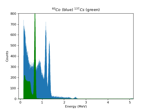
Working with MCA Data

When you do experiments that use a Multi Channel Analyzer (MCA) such as the Maestro program of Ortec (e.g. in the Compton scattering experiment). You save the spectra as ASCII (.SPE) files. You can load these files into python as histograms as follows ( I assume the spectrum name is co_60_cal.Spe ):

In [70]: co = B.get_spectrum('co_60_cal.SPE')
In [71]: cs = B.get_spectrum('cs_137_cal.SPE')

This function returns a histogram which I named co in this example. You can plot it using the standard function (co.plot()). Often you want to focus on a smaller region of the spectrum. This can be done by setting a window with the function set_window as follows.

In [72]: clf()                        # clear the figure
In [73]: co.set_window(200., 310.)
In [74]: co.plot(); show()

Now you see only the region between channels 200 and 310. The window can be cleared with the command clear_window(). You can perform all the functions described above for histograms. Fitting a gaussian is especially useful in order to precisely determine the location of a peak. This is useful for calibrating the spectra that you have taken and is described below.

Energy Calibration

An energy calibration is necessary in order to convert the channel number in your spectrum (histogram) to energy. For this you need to determine the parameters of a function (linear or polynomial) using calibration spectra where the energy of the various peaks are known. In most cases one can assume a linear relationship between channel number and energy.

The procedure is as follows:

• For each known peak fit a gaussian to the top part of each peak. This determines the peak position.

• Create an array containing the fitted peak positions and call it pos

• Create an array containing the corresponding known energies of the peaks and call this array energy. The energy you can get from the literature or the source box. Make sure that the elements in the two arrays correspond to each other.

• Another possibility would be to create a data file (cal.data) and place these calibration data there. Then you can load the data from the file.

• Perform a linear fit as follows:

  In [75]: cal = B.linefit(pos, energy)
  

  You have now an object called cal that contains the calibration fit and the function that converts the channel number to an energy.

• Load the spectrum again (preferably with a different name) and apply the new calibration:

  In [76]: co_cal = B.get_spectrum('co_60_cal.SPE', \
                    calibration = cal)
  In [77]: cs_cal = B.get_spectrum('cs_137_cal.SPE', \
                    calibration = cal)
  

(The backslash means for python that the next line belongs to the first one.) The two new histograms co_cal and cs_cal have now calibrated x-axis. Also note that the statement calibration = cal.line tells the function get_spectrum to use the the function cal.line to convert channels to energy. If you leave this statement off no calibration will be applied.

Below is an example of the two spectra plotted on top of each other.

(Source code)

Background Subtraction

From the Compton experiment you should always have two spectra. One taken with the target and one without. We call the spectrum taken without the target the background spectrum. In order to determine the effect of the target you need to subtract the contribution of the background from the spectrum with the target. First you load the two spectra and apply the energy calibration:

In [78]: cs_tar = B.get_spectrum('cs_45deg_target.SPE',\
                  calibration = cal)
In [79]: cs_bck = B.get_spectrum('cs_45deg_empty.SPE', \
                  calibration = cal)

Here I assumed that cs_45deg_target.SPE is the file containing the data with target and cs_45deg_empty.SPE is the one for the background. Now do:

In [80]: cs_sig = cs_tar - cs_bck
In [81]: clf()
In [82]: cs_sig.plot()

cs_sig contains the signal due to the target. This is the subtracted spectrum. clf() clears the potting window and cs_sig.plot() draws the result. Now you are ready to determine the energy of the scattered photons.

General Linear Fitting

Previously you have encountered fitting of a line and a polynomial to experimental data. Both of these functions are linear in their parameters which makes the least square minimization especially easy. The method can be generalized to fit a function of the form:

\(F(x) = \sum_n a_n f_n(x)\)

where the \(f_n(x)\) are arbitrary functions. To fit such an expression to experimental data we use the function gen_linfit which stands for general linear fit. You need to supply the list of functions. If the functions are relatively simple you can use the so-called lambda function definition in python which allows you to define a function in one line:

f = lambda x: sin(x) (return)

here lambda is a python keyword, followed by the definition of the independent variable ( in this case x) the expression to the right of the colon is the function. In the example above we therefore defined the function \(f(x) = sin(x)\).

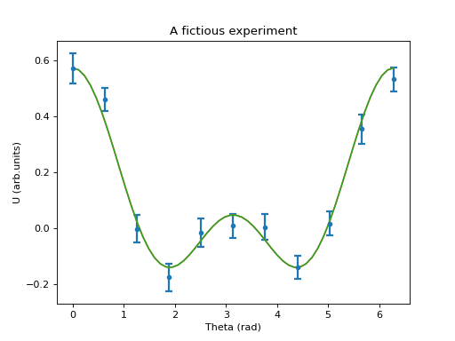
As an example let’s fit the expression:

\(f(x) = a_0 + a_1 cos(x) + a_2 cos(2 x)\)

to the data given by:

In [83]: x = array([ 0.        ,  0.62831853,  1.25663706,  1.88495559,  2.51327412,
         3.14159265,  3.76991118,  4.39822972,  5.02654825,  5.65486678,
         6.28318531])
In [84]: yexp = array([ 0.57344385,  0.46120388, -0.00214848, -0.17668092, -0.01647612,
         0.0076221 ,  0.00437011, -0.13967365,  0.01691304,  0.35493354,
         0.53339805])
In [85]: sigma = array([ 0.05458054,  0.04165251,  0.04823802,  0.05061557,  0.05109571,
         0.04412829,  0.045951  ,  0.04180152,  0.04169562,  0.05209264,
         0.04291919])

Make a plot of the data with errorbars:

In [86]: B.plot_exp(x, yexp, sigma); show()

Next we define the array of fitting functions using lambda functions:

In [86]: f0 = lambda x:1
In [87]: f1 = lambda x:cos(x)
In [88]: f2 = lambda x:cos(2.*x)

Now we can carry out the fit:

In [89]: fit = B.gen_linfit( [f0, f1, f2], x, yexp, yerr = sigma)

with the result:

In [89]: fit = B.gen_linfit( [f0, f1, f2], x, yexp, yerr = sigma)
chisq/dof =  0.964271036369
parameter [ 0 ] =  0.105955015666  +/-  0.0138090697524
parameter [ 1 ] =  0.263317652532  +/-  0.0189765024267
parameter [ 2 ] =  0.204635671851  +/-  0.0186129715857

The fitted function can now be plotted using

In [90]: fit.plot(); show()

(Source code)

As usual the fit function with the current parameters can be evaluated using fit.func(x)

In [91]: fit(3.5)
Out[91]: array([ 0.01364473])

You can access the fitted parameters as follows:

\(a_0 =\) fit.par[0], \(a_1 =\) fit.par[1], \(a_2 =\) fit.par[2]

The parameter uncertainties are accessed via:

\(\sigma_{a_0} =\) fitp.sig_par[0], \(\sigma_{a_1} =\) fitp.sig_par[1], \(\sigma_{a_2} =\) fitp.sig_par[2]

General Non-Linear Fitting

In this case the fitting function is not a linear function of the parameters to be found which requires an iterative procedure to find the minimal value of \(\chi^2\). There are many different methods available to minimize \(\chi^2\), the one used here is based on the Levenberg-Marquardt method. In this case it is important that the parameters have reasonable initial values or it is not guaranteed that the fit converges and a real minimum is found. You have encountered this type of fitting when you fitted a peak in a histogram. Here you will find how to define a general fitting function and how to fit the experimental values using genfit. As an example lets fit a sum of two exponential functions. This would be a situation where two radioactive decays with different lifetimes contribute to your measurement. The fitting function is

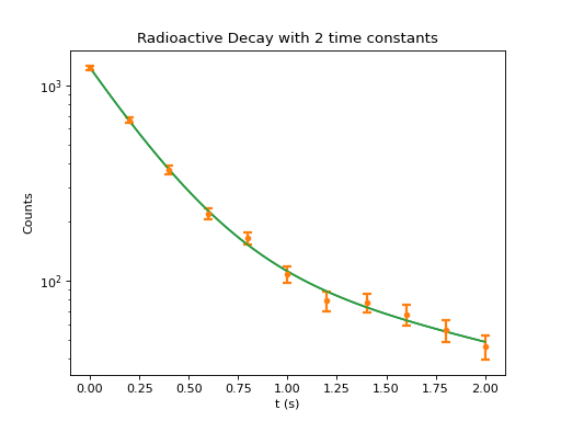
\(F(x) = A_1 e^{-\lambda_1 x} + A_2 e^{-\lambda_2 x}\)

We need to determine the parameters

\(A_1, A_2, \lambda_1, \lambda_2\).

The data are as follows:

In [92]: t = array([ 0. ,  0.2,  0.4,  0.6,  0.8,  1. ,
                     1.2,  1.4,  1.6,  1.8,  2. ])

In [93]: counts = array([ 1235.,   665.,   369.,   221.,
                           165.,   108.,    79.,    77.,
                            67.,    56.,    46.])

In [94]: sigma = array([ 34.64101615,  24.92931125,
                         18.70989477,  14.77306954,
                         12.26884392,  10.62021419,
                         9.46275219,   8.58402083,
                         7.8676807 ,   7.25221607,
                         6.7053333 ])

First we need to define the parameters to be fitted, using the Parameter object:

In [95]: a1 = B.Parameter( 1., 'A1')
In [96]: a2 = B.Parameter( 1., 'A2')
In [97]: lam1 = B.Parameter( 1., 'lambda1')
In [98]: lam2 = B.Parameter( 1., 'lambda2')

It is always a good practice to give your variables and objects names that correspond as closely as possible to the names of the quantities they represent. The statements above do three things:

1. they create the parameter object (a1)

2. they assign an initial value to it (1.) and

3. they also assign a printable name (A1).

Check the capabilities of the parameters by entering the following:

In [99]: a1
Out[99]: <LT_Fit.parameters.Parameter instance at 0x22ea788>

In [100]: print( a1 )
A1 = 1.0 +/- 0.0

In [101]: a1()
Out[101]: 1.0

In [102]: a1.set(10.)
In [103]: print( a1 )
A1 = 10.0 +/- 0.0

In [104]: a1.get()
Out[104]: ('A1', 10.0, 0.0)

As you can see, the print statement prints the name of the parameter, its current value and its error. Calling the parameter like a function returns its current value. This is used when defining the fitting function. The set function is used to assign or change its value and the get function returns all its information in a tuple.

We are now ready to define the fitting function:

In [105]: def f(x): return ( a1() * exp(-lam1()*x) + a2() * exp(-lam2()*x) )

Note: each parameter must have () attached. You need to press

return twice in this case.

After defining the fitting function we are ready to perform the fit:

In [106]: F = B.genfit(f, [a1, lam1, a2, lam2], x = t, y = counts, y_err = sigma)

The arguments are as follows:

Argument	Meaning
f	the fitting function
[a1, lam1, a2, lam2]	the list of the parameters used in the fitting function
x = t	sets t to be the independent variable
y = counts	set counts to be the experimental values to be fitted
y_err = sigma	set sigma to be the uncertainties for each measurement

If you are lucky, the end result looks something like:

----------------------------------------------------------
fit results :
----------------------------------------------------------
chisquare =  3.26261615416
red. chisquare =  0.466088022023
parameters:
parameter  0  :  A1 = 1094.3509 +/- 57.7375
parameter  1  :  lambda1 = 3.6206 +/- 0.3119
parameter  2  :  A2 = 143.7352 +/- 56.5435
parameter  3  :  lambda2 = 0.5485 +/- 0.2298

It might be tricky in the beginning to get a good fit right away. In this case you can also fit only part of the parameters in the function. In the example we fit only the parameters of the first term (a1, lam1) and keep the parameters of the second term (a2, lam2) fixed

In [107]: a1.set(1.)      # reset a1 to 1
In [108]: lam1.set(1.)    # lambda1 back to 1
In [109]: a2.set(0.)      # a2 = 0: second term does not contribute
In [110]: lam2.set(1.)
In [111]: F1 = B.genfit(f, [a1, lam1], x = t, y = counts, y_err = sigma) # fit only a1 and lam1

The in the second step, a1 and lam1 remain constant and only a2 and lam2 are fitted

In [112]: F2 = B.genfit(f, [a2, lam2], x = t, y = counts, y_err = sigma) # fit only a2 and lam2

This should give you a good initial parameter guess. In the last step you fit all parameters:

In [113]: F = B.genfit(f, [a1, lam1, a2, lam2], x = t, y = counts, y_err = sigma) # fit all

This should give you an output similar the one shown previously.

You can plot the exp. data and the fitted values using

In [114]:  B.plot_exp(t, counts, sigma)
In [115]:  F.plot(); show()

(Source code)

The fitting function with its current parameter values can be accessed via F(x) . An example to plot the differences between the fit and the experimental values:

In [116]: d_counts = counts - F(t)
In [117]: clf()
In [118]: B.plot_exp(t, d_counts, sigma); show()

Goodness of a Fit, how to interpret \(\chi^2\)

The quantity \(\chi^2\) is a measure of how well your fitted curve agrees with your experimental data. For a detailed discussion of this quantity please refer to good statistics texts on data analysis such as e.g Data Reduction and Error Analysis for the Physics Sciences by P.R.Bevington and D.K Robinson (a classic) or An Introduction to Error Analysis: The Study of Uncertainties in Physical Measurements by J.R. Taylor or Statistics for Nuclear and Particle Physicists my Louis Lyon and many more. There are of course also considerably more advanced books which you might want to consider later in your career.

The fitting procedures described above are based on least square fitting where the quantity:

\[\chi^2 = \sum_{i=1}^{N}\left[\frac{(y_i-y^{fit}_i(a_1,\dots a_m))}{\sigma_i}\right]^2\]

is minimized by varying the (fit-)parameters \(a_1,\dots a_m)\). The so-called reduced \(\chi^2_{red}\) is defined as

\[\chi^2 = \frac{\chi^2}{(N-m)}\]

and the quantity \(N - m\) is called the number of degrees of freedom of the fit. If your data are well described by your model function \(y^{fit}(x)\) then \(\chi^2_{red}\approx 1.\). All fit functions also calculate a quantity loosely called the confidence level which corresponds to the probability that a new set of data will result in a \(\chi^2\) value which is larger than the one you obtained. If your error estimates are correct and the function you selected really describes the data then this probability should be around 0.5. This quantity is automatically calculated in your fit and called \(CL\). E.g. for the linear fit described in the beginning you could view it by entering

In [45]: fit.CL

When \(CL\) is close to 1, it indicates that your error estimates are probably too large (your \(\chi^2_{red}\) value typically is small) and when \(CL\) is very small it indicates the model you use does not represent the data very well (typically \(\chi^2_{red} >> 1\))

Caution: Neither the \(\chi^2_{red}\) nor the \(CL\) value can identify the exact problem of a fit.

Fitting data without Errors

Sometime you might not have information on the uncertainties (errors) of the individual data points that you are using in a fit. In this case the value of \(\sigma_i\) is set to 1 for all data points. In this case you cannot interpret the \(\chi^2\) value as above, but you get an estimate of the common error of your measurements. You can look at it by doing:

In [45]: fit.common_error

Note: This quantity is only calculated if you did not provide measurement errors.