26. Transistor Characteristics
26.1. Background
The transistor ranks as one of the greatest inventions of 20th century technology. It finds application in virtually all electronic devices from radios to computers. Integrated circuits typically contain millions of transistors, formed on a single tiny chip of silicon. Two of the basic uses of a transistor, which will be explored in this experiment, are as an amplifier and as a switch.
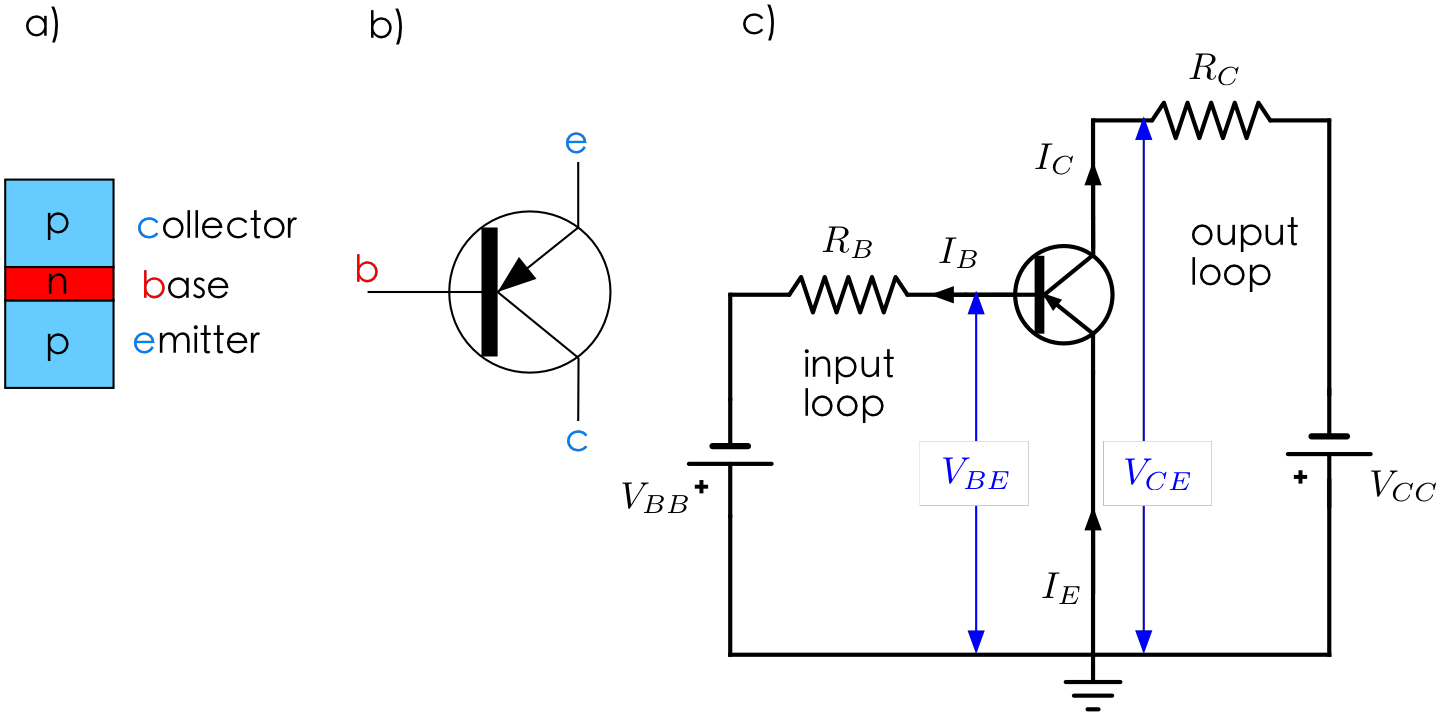
Fig. 26.1 a) Schematics of the pnp transistor. b) Circuit symbol (note the emitter, base and collector symbols) c) The common emitter circuit.
The php transistor, shown in Fig. 26.1 (a) contains three distinct regions, a p-type ”emitter”, an n-type “base” and a p-type “collector”, which together form two pn junctions. In a typical amplifier circuit, voltages are supplied so that the emitter-base junction is forward-biased and the collector-base junction is reverse-biased. This means that \(V_{CE} > V_{BE}\). Fig. 26.1 (c) illustrates a “common emitter” circuit, so called because the emitter is common to the input circuit on the left and the output circuit on the right.
Consider first the forward-biased emitter-base junction. The doping of the emitter is made much heavier than that of the base so that positive holes from the emitter form almost all of the current, \(I_E\), from emitter to base. The base, being lightly doped, does not have many electrons available for recombination with these holes to form neutral atoms. It is also very narrow (\(< 1 \mu m\)) making it easy for a large fraction, \(\alpha\), of the holes to diffuse across to the collector-base junction where the junction voltage accelerates them into the collector region to form the collector current, \(I_C\).
Thus,
The remaining fraction, \((1-\alpha)\), of holes leave the base through the external connection to form the base current, \(I_B\), where
The “current gain”, \(\beta\), of the transistor is defined by
For typical transistors, \(0.9 \leq \alpha \leq 0.995\) , giving values of \(10 \leq \beta \leq 200\). Thus we have a “current amplifier”, in that a small change in \(I_B\) will cause a large change in \(I_C\). The “voltage gain”, \(A_V\), is the ratio of the voltage drop, \(I_C R_C\), across the output resistor, \(R_C\), to the voltage, \(V_{BB}\), of the input source:
Applying the loop theorem to the input circuit in Fig. 26.1 (c), and assuming \(I_E \approx I_C = \beta I_B\), one obtains
where \(r_B\) is the resistance of the emitter-base junction. By a suitable choice of resistors, an appreciable voltage amplification may be obtained.
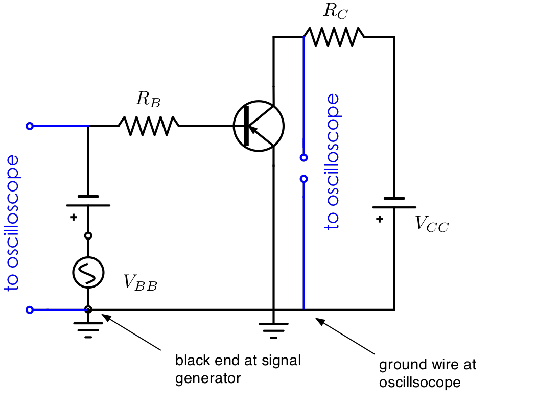
Fig. 26.2 The AC amplifier circuit.
Fig. 26.2 shows how the transistor may be used as an AC amplifier to amplify a small signal from a signal generator (e.g. the output of the DAC, a digital to analog converter, of a CD or MP3 player). The two batteries in the circuit behave like large capacitors with impedances \(1/\omega C \approx 0\). Once again the voltage gain is given by equation (26.5). However, this is a simplified situation. In reality, the transistor junctions possess capacitance, and the corresponding reactances are frequency dependent. Thus we can expect Av to be a function of frequency.
26.2. Experiment
26.2.1. Preliminary Studies
Set up the circuit shown in Fig. 26.1 (c) using the power supply outputs for
the voltages \(V_{BB}\) and \(V_{CC}\). Note the symbols
e, b and c denoting the transistor connections. Use a
\(3000\Omega\) resistor for \(R_B\) and a \(220\Omega\)
resistor for \(R_C\). Turn the supply outputs to zero then turn on
the unit. Set one of the digital meters to the 20 V-DC range and
connect it to measure \(V_{CC}\) (+ lead to ground on the
transistor board). Adjust \(V_{CC}\) to approximately 15
V. Reconnect the meter to measure \(V_{CE}\). This should also
read 15 V, indicating \(I_C = 0\). Connect the second meter to measure
\(V_{BE}\) (also with the + lead to ground). Slowly increase \(V_{BB}\) up to 2 V and
note \(V_{CE}\) decreasing, indicating an increasing \(I_C\). Your amplifier is
now working.
26.2.2. DC operation
Set \(V_{BB}\) to 0.75 V. Reconnect the meter to measure \(V_{BE}\) and calculate
Now reconnect the meter to measure \(V_{CC}\). (The first meter should still be measuring \(V_{CE}\).) Adjust \(V_{CC}\) to 1, 3, 5, …. 15 V and calculate corresponding values of
Repeat with \(V_{BB}\) = 0.90 and 1.05 V. Plot on a single graph \(I_C\) (y-axis) vs \(V_{CE}\); (x-axis) for each value of \(I_B\). The “operating region” of the transistor is where the curves level off. Determine \(\beta\) for the middle curve at \(V_{CE}\) = 3 V. Is \(\beta\) generally constant?
26.2.3. Transistor as a switch
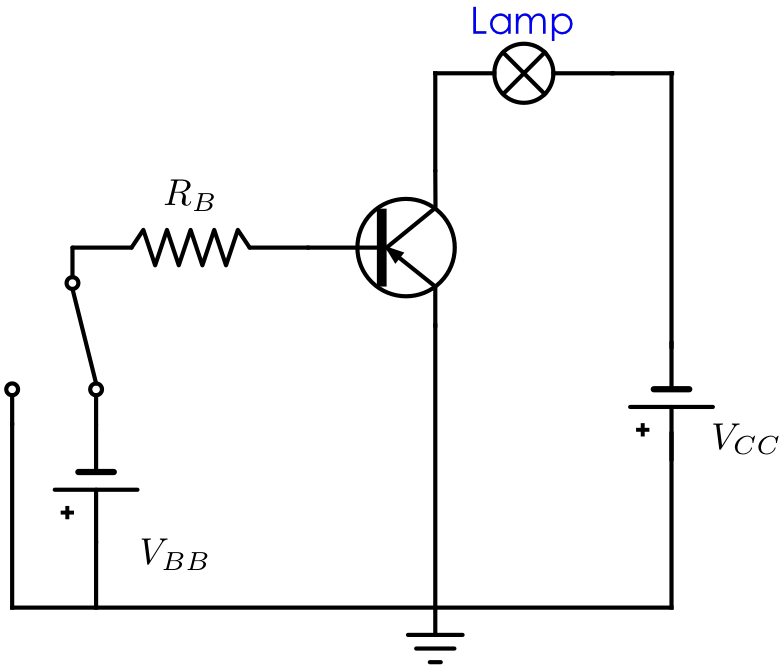
Fig. 26.3 The transistor as a switch.
Reconnect the meters to measure \(V_{CC}\) and \(V_{BB}\), set \(V_{CC}\) to 6 V and decrease \(V_{BB}\) to zero. Replace \(R_C\) with the light bulb. Slowly increase \(V_{BB}\) until the bulb is at maximum intensity. Connect the two-way switch as shown in Fig. 26.3. Note the effect of operating the switch. Measure \(V_{BE}\) to determine the very small current \(I_B\) that you are turning on and off to control the much larger current (~ 1A) through the light bulb. ,
26.2.4. AC Amplifier
Reconnect the circuit of Fig. 26.1 (c) with the meters to measure \(V_{CC}\) and \(V_{CE}\). Increase \(V_{CC}\) to 15 V and turn \(V_{BB}\) down to zero. Increase \(V_{BB}\) until \(V_{CE}\) = 7.5 V. Connect the signal generator in series with \(V_{BB}\) as shown in Fig. 26.2 and adjust it to 100Hz. Connect the oscilloscope also as in Fig. 26.2 WITH THE BLACK LEADS TO GROUND ON THE TRANSISTOR BOARD FOR BOTH CONNECTIONS. Observe the input and output waveforms. Note that adjusting \(V_{BB}\) causes distortion of the output waveform. Can you explain this? From the ratio of peak-to-peak voltages, determine \(A_V\) for frequencies of 100 Hz, 1 kHz, 10 kHz and 20kHz. Would this amplifier be good as an audio-amplifier? Replace \(R_C\) with a \(120\Omega\) resistor and note the effect on \(A_V\). Is this an expected result?