25. High Temperature Superconductor

25.1. Background

Superconductivity was first discovered in 1911 in metals such as mercury, lead and bismuth. The “critical temperatures”, \(T_c\), at which these metals changed from being ordinary conductors with finite resistance to superconductors with zero resistance, was very low. For example, \(T_c\) for mercury is 4.2 K, achievable with liquid helium. The so-called high temperature superconductors were discovered in 1986. In terms of composition, they can be classified as metallic ceramic oxides. Two are available for this experiment, \(YBa_2Cu_3O_7\) and \(Bi_2CaSr_2Cu_2O_9\). Their advantage is that they become superconductors at temperatures exceeding that of liquid nitrogen (\(77 ^\circ K\)), which is relatively cheap and plentiful.

The behavior of the original “Type 1” superconductors is explained by the BCS theory in which pairs of electrons form bound states called “Cooper pairs”. It is uncertain, however, whether the BCS theory is applicable to the high \(T_c\) superconductors. A more promising approach is the “Resonant Valence Bond” theory, the basis of which is familiar to organic chemists. < In addition to being a perfect conductor, a superconductor is a perfect diamagnet. Recall that diamagnetism arises when an external magnetic field alters the orbital motion of an electron and hence the associated orbital dipole moment. The total dipole moment, which includes electron spin dipole moments, then opposes the external field. The result is the Meissner Effect - a strong repulsion between the superconductor and the magnet supplying the external field.

In this experiment you will demonstrate the Meissner Effect and also determine the variation in resistance of a superconductor with temperature.

25.2. Procedure

You will be using liquid nitrogen in order to achieve temperatures at which superconductivity is observable. At normal atmospheric pressure, liquid nitrogen boils at \(77 ^\circ K\) (\(-196 ^\circ C\)). Since the insulated containers (Dewar bottles) are not pressurized, this will be the liquid nitrogen temperature. Be very careful when handling it. Wear safety glasses and avoid splashing when pouring it from the Dewar bottle into another container.

25.2.1. The Meissner Effect

Identify the bismuth-based superconducting disk. Pour a small amount of liquid nitrogen into the shallow depression in the styrofoam block to a depth of about a quarter of an inch. When the liquid has stopped boiling, use the plastic tweezers to place the superconducting disk in it (see Fig. 25.1). The top of the liquid should be flush with the surface of the disk. When the boiling has again subsided, use the tweezers to float the cubical rare earth magnet above the disk. The magnet should float a few millimeters above the surface of the disk. This is the Meissner Effect. Now remove the magnet and place the yttrium-based disk in the liquid nitrogen. Add more liquid if necessary. Then rapidly remove both disks from the liquid nitrogen, place them on paper towels and float magnets above each. Wait until each disk has stopped exhibiting the Meissner Effect. What do you conclude about their relative critical temperatures?

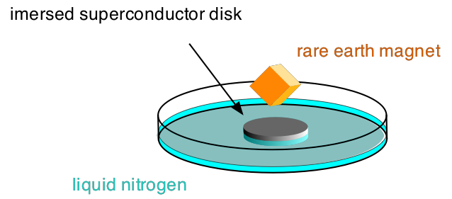
Fig. 25.1 Setup for observing the Meissner effect.

IMPORTANT: When they are removed from the liquid, the disks will acquire a coating of frost. Before returning them to their plastic bags they must be thoroughly dried with paper towels and a hot-air gun. Do not overheat the disks by holding the gun too close.

25.2.2. Variation of Resistance as a Function of Temperature

The measure a resistance with high precision, ones uses a so called four-point-probe. The principle with the circuitry is shown in Fig. 25.2.

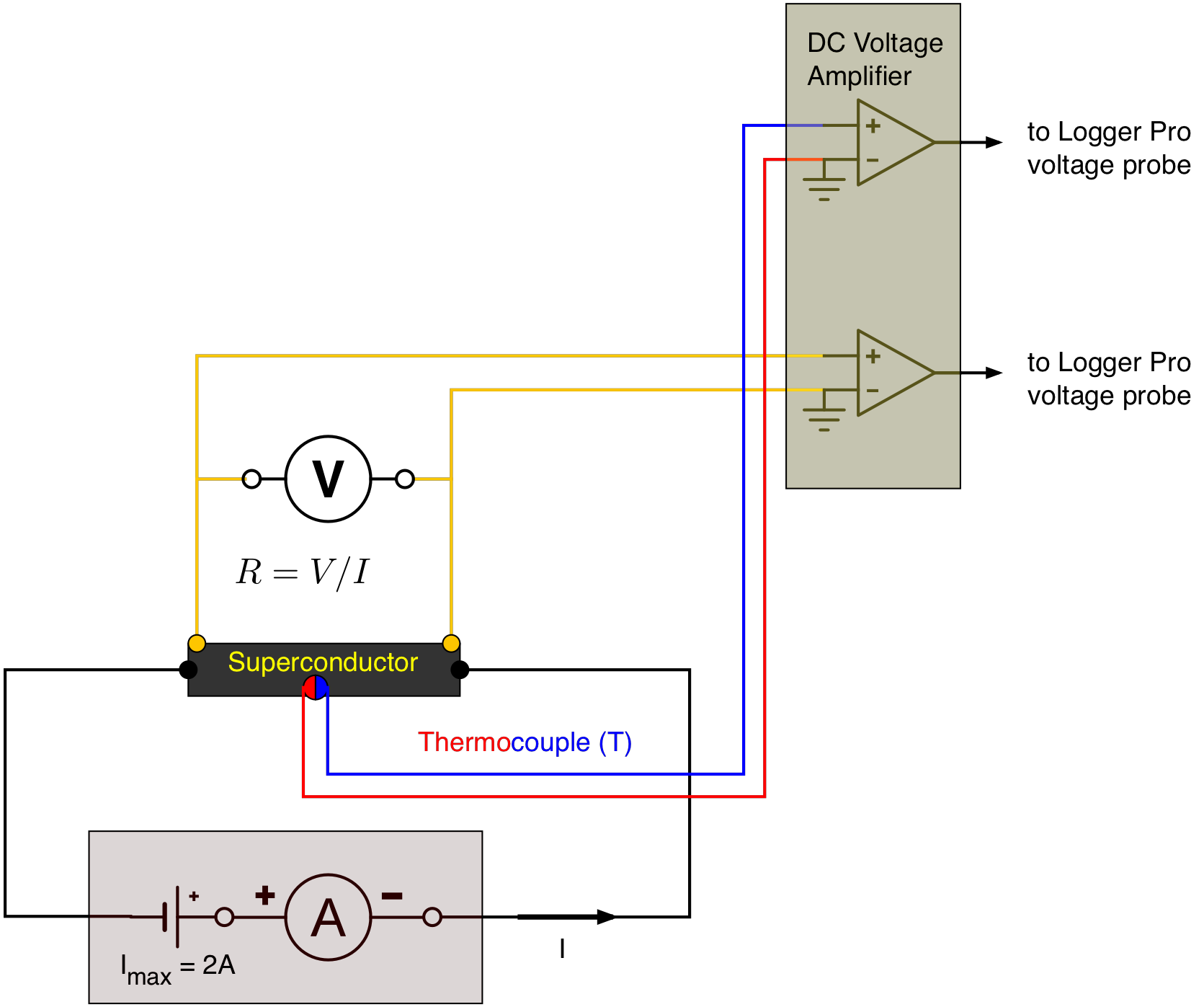
Fig. 25.2 Setup of the four-point probe to measure the resistance as a function of temperature.

The superconducting material is connected to the power supply via the black leads. When a current flows through the yellow connectors which are directly connected to the material are used to measure a potential difference. Measuring a potential difference requires very small currents and therefore the additional resistances between the leads and the connectors for the voltage probe do not affect the resistance measurement. The temperature of the sample is measured using a thermocouple, delivering a temperature dependent small voltage. The voltage across the superconducting sample will also be quite small. In order to be able to record these small voltages using the Logger Pro they need to be amplified by a factor of either 100 or 1000 and a DC offset needs to be adjusted.

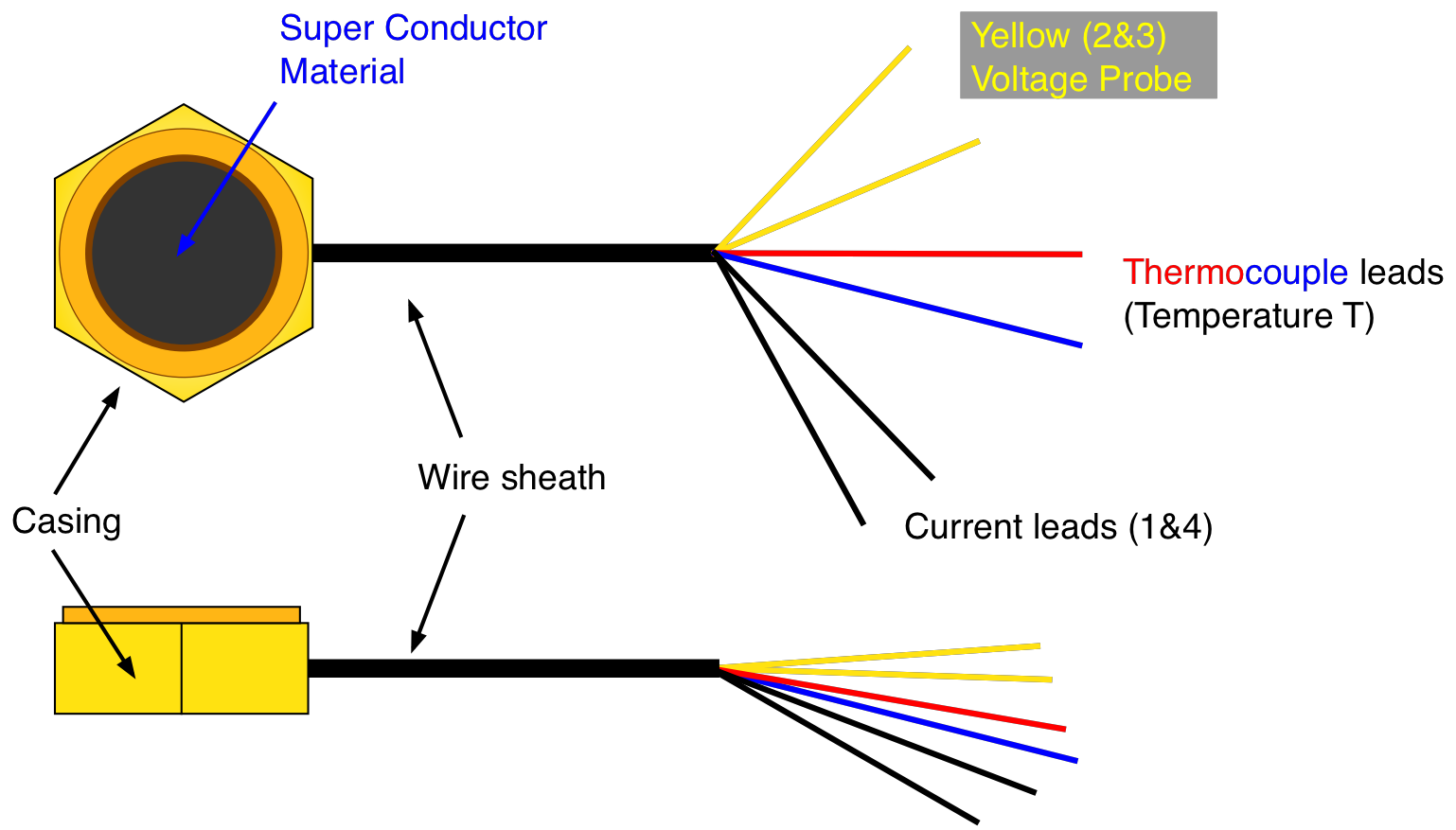
Fig. 25.3 Schematic of the four-point probes with their leads.

Identify the two “Superconducting 4 Point Probes”. The yttrium- and bismuth-based probes, shown schematically in Fig. 25.3, have a “Y” and a “B”, respectively, stamped into the brass casing. Fig. 25.2 shows the electrical connections for resistance measurements. Note that if the superconducting disk had only two probes, 1 and 4, and the voltmeter was connected across the power supply and ammeter, the measured voltage would include the contact potentials between the metal probes and the superconducting material. To put it another way, the calculated resistance would include the contact resistance.

Set up the circuit as in Fig. 25.2 using the bismuth-based 4 point probe (note that the 4 point probe actually has 6 wires).

1. First connect the red and blue thermocouple leads to a digital voltmeter set on the mV scale and check that the digital voltmeter is giving a reading. THen connect it to one of the inputs of the voltage amplifier and adjust the gain and offset in such a way that the amplified voltage is proportional to the real voltage. [The table in the back of this lab will let you convert between the potential difference across the thermocouple and the temperature of the disk.]

2. Connect the ammeter in series with the power supply. NEVER EXCEED 0.5 AMPS THROUGH THE SUPERCONDUCTOR. Adjust the current to 0.25 A as measured through the ammeter.

3. Connect probes 2 and 3 to the third multimeter to measure the voltage across the disk as shown in Fig. 25.2. Adjust the scale to read millivolts. Then connect it to the DC amplifier and adjust again the gain and offset to get a proportional reading using the LoggerPro voltage probes.

Pour some liquid nitrogen into the insulated cup container. When boiling has ceased, completely immerse the 4 point probe, lowering it carefully by its connecting leads. Note that these will become brittle and fragile at liquid nitrogen temperatures.

Now carefully remove the 4 point probe from the liquid nitrogen and wrap it in a few sheets of paper towel to insulate it. Start recording the voltages of your two voltage probes with LoggerPro. When the temperature has gone some way beyond the critical temperature you can stop. Use the thermocouple calibration and the proportionality constant from the amplifier to calculate the temperature. Plot the resistance as a function of temperature.

Thoroughly dry the bismuth-based 4 point probe and then repeat the experiment with the yttrium-based 4 point probe. Discuss the shapes of the two graphs and from them, determine the values of \(T_c\).