24. Stefan-Boltzmann Law

24.1. Background

A body at a certain temperature continuously absorbs and emits electromagnetic radiation. If it absorbs more energy that it emits its temperature will increase and if it emits more energy than it absorbs it’s temperature will decrease. When it is in a thermal equilibrium with its surroundings then it absorbs the same amount of power as it emits. An ideal body that absorbs all electromagnetic radiation that impinges on its surface is called a black body. The spectrum of the radiation emitted by a black body is entirely determined by its temperature and independent of its composition.

In 1900, Max Planck obtained his famous blackbody formula that describes the energy density per unit wavelength interval of the electromagnetic radiation emitted by a blackbody at a temperature \(T\) :

(24.1)\[u(\lambda,T) = \frac{8\pi h c}{\lambda^5(e^{hc/\lambda kT} - 1)}\]

where \(\lambda\) is the wavelength, \(T\) is the temperature of the body, \(k\) is the Boltzmann constant, \(h\) is Planck’s constant and \(c\) is the speed of light.

A good realization of a black body is a cavity with a small hole through which a small amount of radiation can exit (for observation) without disturbing the thermal equilibrium inside. If one assumes for simplicity that the cavity is made out of an electric conductor, one can show that only certain standing transverse electromagnetic waves are allowed. Each electromagnetic wave behaves statistically like a harmonic oscillator of a certain frequency. While a classical oscillator can contain any amount of energy, in order to obtain his result, Planck had to assume that a harmonic oscillator is quantized i.e. can only contain a total amount of energy given by \(E=n\hbar \omega_0\) where \(n = 1,2, ...\). In addition he assumed for a given type of oscillator (characterized by \(\omega_0\)) that the ratio of the number of oscillators in a state \(j\) to the number of oscillators in another state \(i\) is given by \(\frac{N_i}{N_j} = e^{-\Delta E/kT}\) where \(\Delta E = E_i - E_j\). Using this assumption the average energy per oscillator is:

(24.2)\[ \begin{align}\begin{aligned}<E> = \frac{E_{tot}}{N_{tot}} = \frac{N_0\hbar\omega_0\left( 0 + x + 2x^2 + 3x^3 + ...\right)}{N_0\left(1+x+x^2+x^3 + ...\right)}\\x = e^{-\hbar\omega_0/kT}\end{aligned}\end{align} \]

evaluating the infinite sums gives:

(24.3)\[<E> = \frac{\hbar\omega_0}{e^{\hbar\omega_0/kT} - 1}\]

He further assumed that when an oscillator changes from an initial state \(i\) to a final state \(f\) he emits (or absorbs) radiation with a frequency such that \(E_f - E_i = 2\pi \hbar \omega\). Since the electromagnetic radiation is confined in a cavity with a volume \(V\) the number of oscillators with a frequency between \(\nu\) and \(\nu + d\nu\) is given by:

(24.4)\[dZ = \frac{8\pi V \nu^2}{c^3} d\nu\]

leading to an energy density per unit frequency inside the cavity of

(24.5)\[u_{\nu} = \frac{8\pi h \nu^3}{c^3\left( e^{h\nu/kT} -1 \right)}\]

corresponding to (24.1) when \(\nu\) is replaced by \(\lambda\). The surface intensity (per unit solid angle) is obtained as follows:

(24.6)\[ \begin{align}\begin{aligned}I(\nu, T) = \frac{c}{4\pi} u_{\nu} = \frac{2 h \nu^3}{c^2\left( e^{h\nu/kT} -1 \right)}\\I(\lambda, T) = \frac{2 h c^2}{\lambda^5\left(e^{hc/\lambda kT} -1 \right)}\end{aligned}\end{align} \]

The total power per unit area and unit solid angle, a \(P\), radiated by a blackbody is found by integrating \(I(\lambda, T)\) over the entire wavelength range from zero to infinity. When this is done, we obtain the Stefan-Boltzmann law:

(24.7)\[ P = \sigma T^4\]

where the \(\sigma\) is the Stefan-Boltzmann constant. For an incandescent solid, the ratio of the energy radiated to that from a true blackbody at the same temperature is called the emissivity, \(e\), a number which is always less than one.

The goal of this experiment is to investigate the relationship between \(E\) and \(T\) for the tungsten filament in an ordinary lamp to see how close it behaves like a black body radiator. The emissivity of tungsten is not quite constant but decreases with increase in wavelength and increases in temperature. The temperature of the filament will be determined from its change in resistance with temperature.

24.2. Experimental Equipment

The setup for this experiment is shown in Fig. 24.1. It consists of a 12V light bulb with a tungsten filament and a radiation detector which produces an output voltage proportional to the detected radiation power (22 mV per mW).

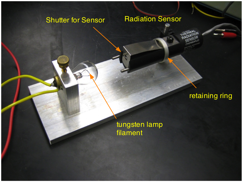
Fig. 24.1 Main parts of the Stefan-Boltzmann experiment. The shutter should be closed when not taking a measurement. It can be kept closed by moving the retaining ring forward.

24.2.1. Radiation Detector

To measure the emitted radiation power a thermopile sensor is used which consists of a series of thermocouples connected alternatively to an active side and a reference side (see Fig. 24.2). The active side typically consists of a very thin layer of material. The output voltage of this series is proportional to the temperature difference between the active layer and the reference layer. The total radiation is absorbed in the active layer where a temperature increase proportional to the absorbed radiation power is detected and converted to a voltage.

Fig. 24.2 Schematic of a thermopile detector. Incoming radiation changes the temperature of the thermocouples in the active layer. The measured voltage is the added voltage of the series of thermocouples in the detector.

The wavelength range for this detector is indicated on its side.

24.2.2. Wheatstone Bridge

For this experiment we will also use a Wheatstone bridge to accurately determine the resistance, \(R_{ref}\), of the lamp filament at room temperature (~ 300K) and the resistance of the wires connecting the lamp to the power supply.

The schematic of this instrument is shown in Fig. 24.3

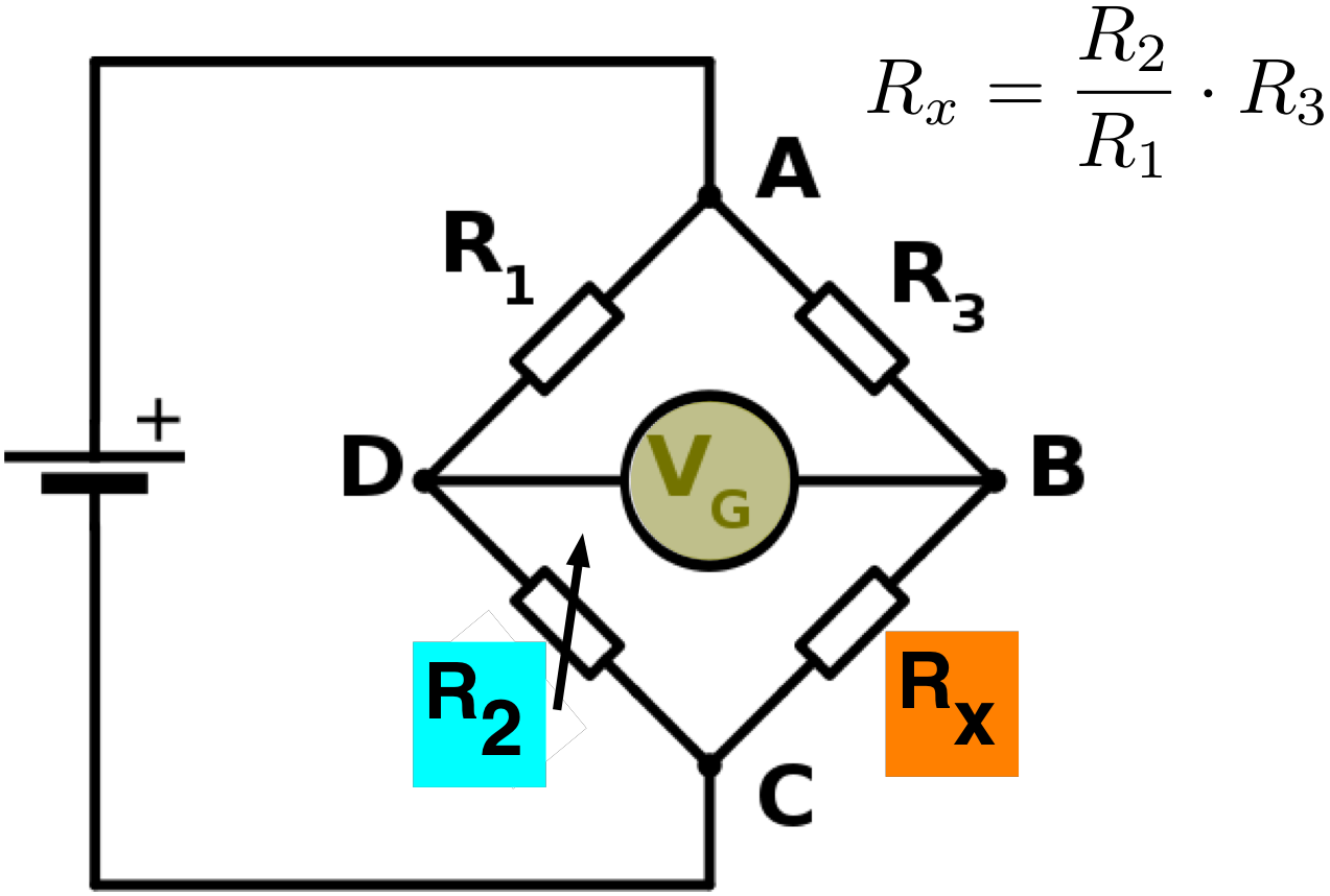
Fig. 24.3 Schematic of a Wheatstone bridge to determine an unknown resistor. Resistor \(R_2\) is adjustable and the other resistors are known except for \(R_x\). \(R_2\) is adjusted until no current is measured in the galvanometer \(V_g\) (the bridge is then called balanced). The resistance \(R_x\) can then be calculated as shown.

The actual instrument with the various controls and connections is shown in Fig. 24.4

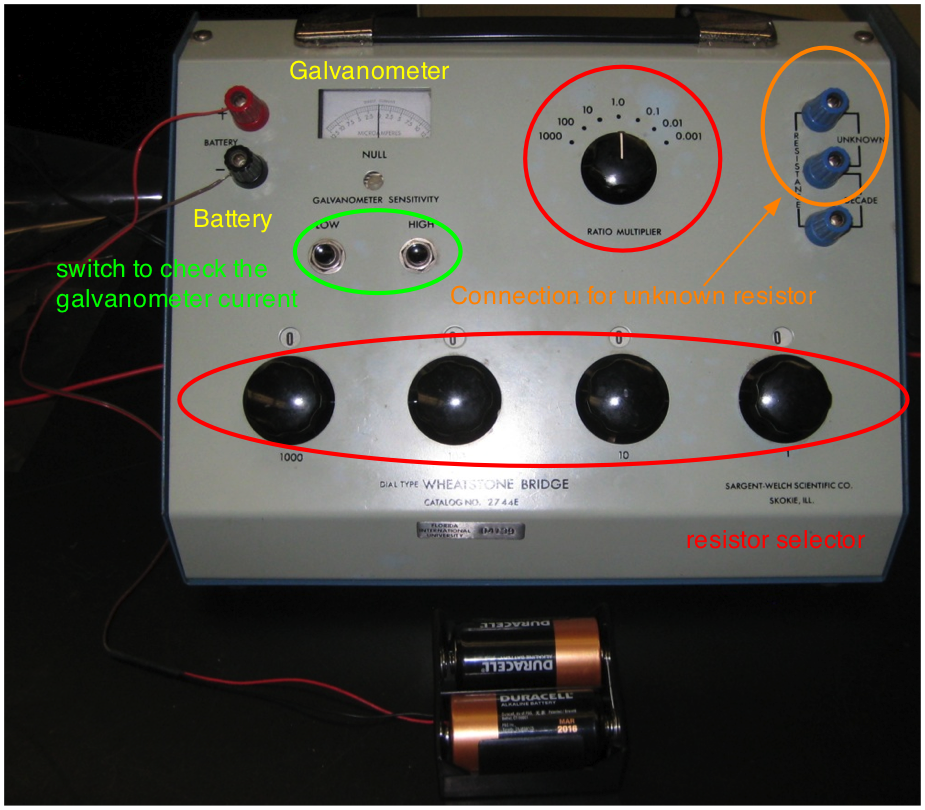
Fig. 24.4 The Wheatstone apparatus used in the experiment with its main controls.

24.3. Experimental Procedure

Use a 3V battery pack as the power supply and first determine the resistance of the lamp connecting leads. A dummy lead of the same total length is provided for this purpose. Then measure the resistance of the lamp plus connecting leads and, by subtraction, obtain the filament resistance alone. These measurements need to be done very accurately as a small error will lead to large errors in filament temperatures.

Connect the radiation sensor (thermopile) to a digital multimeter that should be set on a 100 or 200-millivolt DC range. Connect the lamp to a DC power supply together with an ammeter and voltmeter to record filament current and voltage respectively.

HAVE YOUR CIRCUIT CHECKED BY AN INSTRUCTOR BEFORE SWITCHING ON. NOTE ALSO THAT THE LAMP VOLTAGE SHOULD NEVER EXCEED 12 V.

Measure the distance between the lamp filament and the detector opening. Also record the detector diameter.

For filament voltages of between 1V and 12V in steps of about 1V, record the filament voltage, current and the sensor millivoltmeter reading. Make the latter readings quickly and in between readings, place a reflecting heat shield between the lamp and sensor with the reflecting surface facing the lamp. This will help to keep the sensor at a relatively constant temperature. Note that the millivoltmeter reading, designated “Rad” in Table 1, is proportional to the total power radiated by the lamp.

Measure the temperature in the room (you can read the thermometer from the Franck-Hertz experiment for this) and record it as well.

24.4. Analysis

First you need to determine the filament temperature. To do this we use the known tungsten resistivity as a function of temperature. You can download W_resistivity.data to get a data file with the resistivity information. From this file you can get the resistivity (R) as a function of temperature (T).

First we need to know the resistivity of the tungsten at the current room temperature. To do this you will first read the data an fit a 7-th order polynomial to get R as a function of T:

In [1]: rd = B.get_file('W_resistivity.data')
In [2]: R = B.get_data(rd, 'R')
In [3]: B.get_data(rd,'T')
In [4]: Rf = B.polyfit(T,R, order = 7)

You should get an output like:

chisq/dof =  0.000444541390639
parameter [ 0 ] =  0.786467375234  +/-  0.20463740899
parameter [ 1 ] =  0.00842119057779  +/-  0.00124878972052
parameter [ 2 ] =  3.38132589377e-05  +/-  2.84216959531e-06
parameter [ 3 ] =  -2.98493892381e-08  +/-  3.20401959016e-09
parameter [ 4 ] =  1.58106971254e-11  +/-  1.97223496095e-12
parameter [ 5 ] =  -4.78596183333e-15  +/-  6.73770637135e-16
parameter [ 6 ] =  7.70654530692e-19  +/-  1.19806308507e-19
parameter [ 7 ] =  -5.11638418846e-23  +/-  8.64022222901e-24

Now you can calculate the resistivity of tungsten at your room temperature:

In [5]: R_ref = Rf.poly(295.) # it was assumed that the room is at 295K

We will not be able to directly measure the resistivity of the tungsten filament but its resistance (check your physics book on the difference between resistivity and resistance). The ratio of the filament resistance at different temperatures is dominated by the corresponding ratio of the tungsten resistivity. We therefore need to calculate the ratio of the resistivity at a give temperature to the one at our current room temperature \(R_{rel}(T) = R(T)/R_{ref}\) . Then we fit \(T\) as a function of \(R_{rel}\) again using a 7-th order polynomial:

In [6]: R_rel = R/R_ref
In [7]: Temp = B.polyfit(R_rel, T, order = 7)
chisq/dof =  0.748733057894
parameter [ 0 ] =  35.0101136416  +/-  3.42110385654
parameter [ 1 ] =  288.88629356  +/-  4.42701538565
parameter [ 2 ] =  -32.1923642159  +/-  2.00772236211
parameter [ 3 ] =  5.39380439371  +/-  0.433502793096
parameter [ 4 ] =  -0.535908552352  +/-  0.0498179195972
parameter [ 5 ] =  0.0300782229751  +/-  0.00312310690913
parameter [ 6 ] =  -0.00088651572878  +/-  0.000100685923028
parameter [ 7 ] =  1.06612957893e-05  +/-  1.30509370423e-06

Now you have a function to get the temperature as a function of the resistivity ratio.

1. From your measured data read the current and voltages of the lamp and determine its resistance.

2. Correct the resistance for the lead wire resistances and calculate the resistivity ratios for your measured data.

3. Use the fitted function to determine the filament temperature.

4. Fit a line to the logarithm of the measured power (include its estimated error) as a function of the logarithm of the temperature. What power to you determine from this ?

5. Select only those points where the temperature is larger than about 1500-2000K. And repeat the previous step

6. Make a linear fit of the measured power as a function of \(T^4\). Can you estimate the value of \(\sigma\) in the Stefan-Boltzmann law ((24.7), remember it is the power per unit area of emitter)