27. X-Ray Spectrometer

27.1. Background

In this experiment, X-rays are created in an X-ray tube ( Fig. 27.1) from a copper target and undergo diffraction from a sodium chloride crystal. By measuring the intensity of the reflected X-rays as a function of the scattering angle, the spacing between the atomic planes in the crystal may be determined.

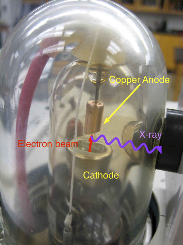
Fig. 27.1 The X-ray tube used in the experiment. Electrons are accelerated from the cathode to the anode.

The X-ray spectrum consists of a continuous part that is due to the acceleration of the electrons in the coulomb field of the copper nuclei and is called “Bremsstrahlung” (translated literally from German it means “braking radiation”). Superimposed on the continuous X-ray spectrum are several sharp lines. In the case of copper, there are two, which are prominent: the K\(\alpha\) and K\(\beta\) lines. These occur when an electron incident on the target removes an inner (K-shell) electron from a target atom and this is replaced by an L-shell or M-shell electron respectively. In the process, the electron making the transition loses energy, which appears as an emitted X-ray photon. The wavelengths of the K\(\alpha\) and K\(\beta\) lines for copper are 1.542 \(\cdot 10^{-10}\) and 1.392 \(\cdot 10^{-10}\) meters respectively.

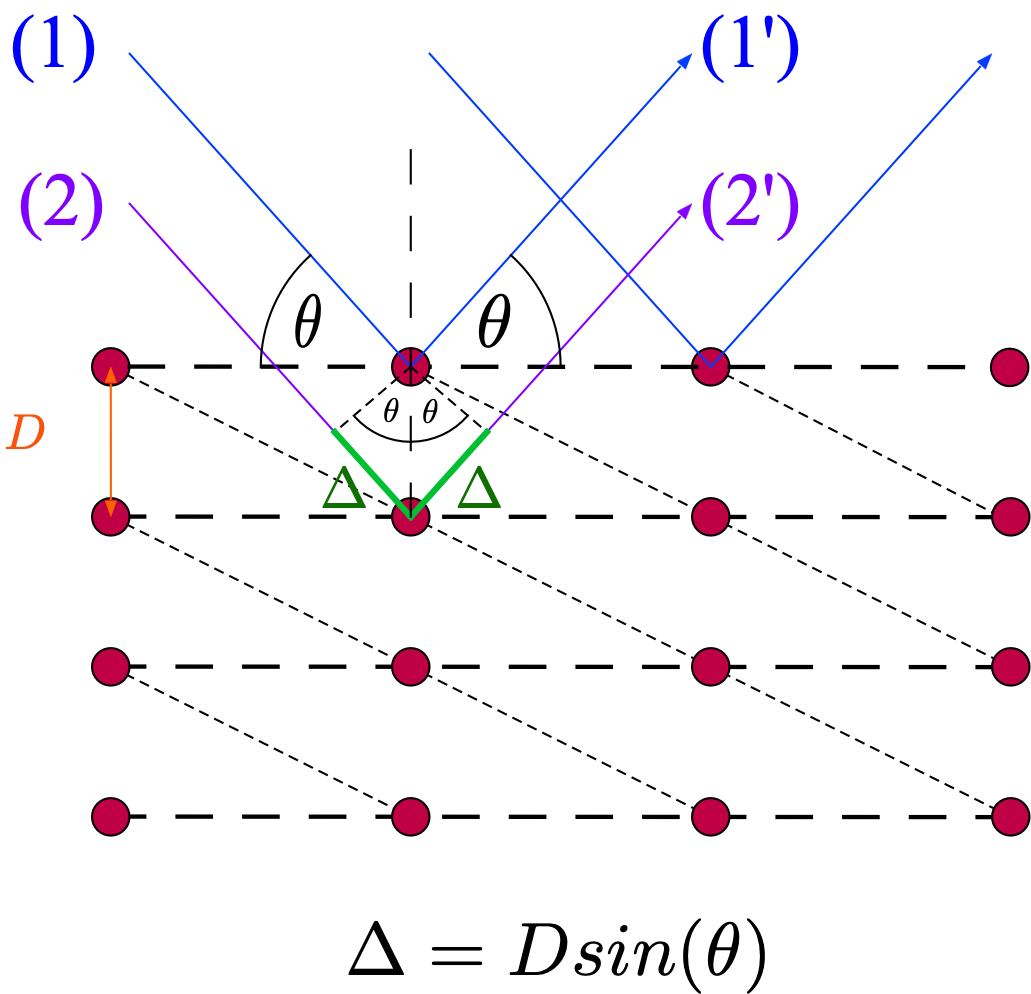
Fig. 27.2 Reflection of X-rays from atomic planes. \(2 \Delta\) is the path length difference between the reflected ray from the top plane (1’) and the reflected ray from the one plane below (2’). The short-dashed lines show another possible set of atomic planes.

A useful model for the formation of diffraction patterns in X-ray diffraction is due to W.H and W.L Bragg (1913). They regarded the crystal to me made of parallel (atomic) planes from which the X-rays are reflected specularly (incident angle equal reflected angle). Only a small fraction of a wave is reflected from each plane and the final superposition of all these reflected waves lead to the observed diffraction pattern. For a single crystal, strong reflection of waves occurs when the so-called Bragg condition is met as shown in Fig. 27.2. Two incident light rays (1) and (2) which are part of the incident plane wave are reflected from the top atomic plane and the one below, respectively. This leads to a path length difference between thwe reflected rays (1’) and (2’) of \(2 \Delta\) where \(\Delta = D sin(\theta)\) and \(D\) is the distance between the atomic planes. The Bragg condition for constructive interference is therefore given by:

(27.1)\[2 D sin(\theta) = n \lambda , n = 1,2, ...\]

Here \(\theta\) is the angle of incidence with respect to an atomic plane and the X-ray wavelength is \(\lambda\). The constructive interference happens between rays that are reflected from different, parallel planes when the total path length difference \(2\Delta\) is \(n \lambda\).

27.2. Pre-Lab Preparation

1. Note that the angle you record during the experiment, let’s call it \(\phi\), is actually \(\phi = 2\theta\), with \(\theta\) being the incident angle appearing in the Braggs Equation \(2d \sin{\theta} = n \lambda\) . For one of the characteristic wavelengths you observed a maximum count rate at \(\phi=30.0\) degrees. Predict where - please! Do NOT answer 60 degrees! - you should be observing the second maximum count rate for that same wavelength. What about the third, and the fourth if it is even possible.

2. Prepare the data files for the coarse and the fine angle measurements.

3. Prepare a small python script to plot the data that your are taking including the estimated errors in the measured counts.

27.3. Experimental Procedure

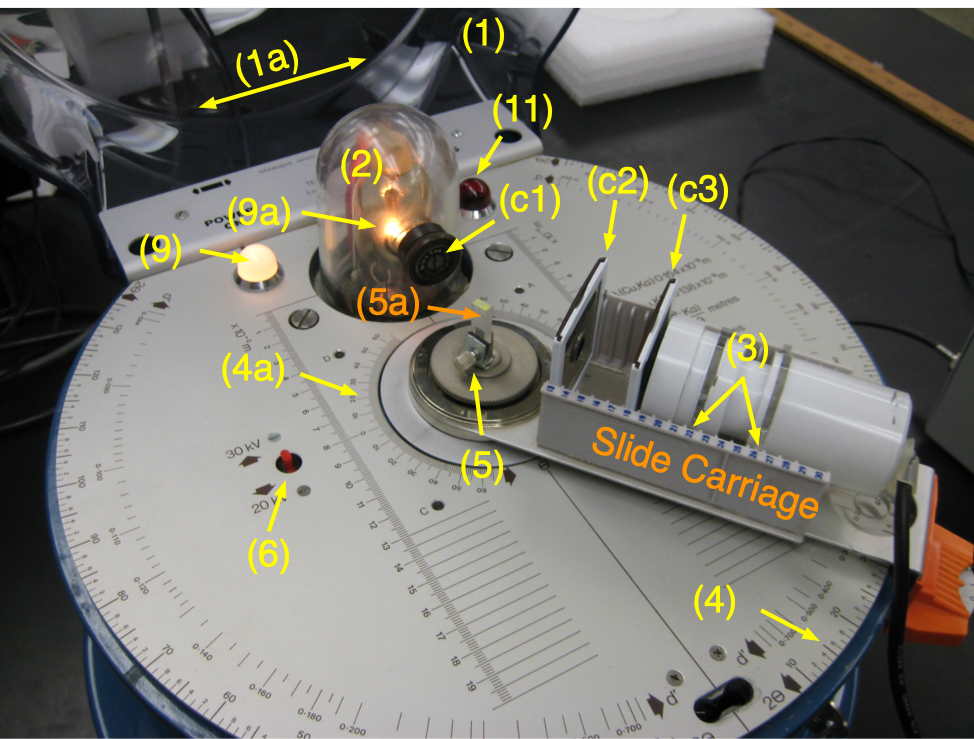
Fig. 27.3 Overview of the X-ray apparatus including its main parts.

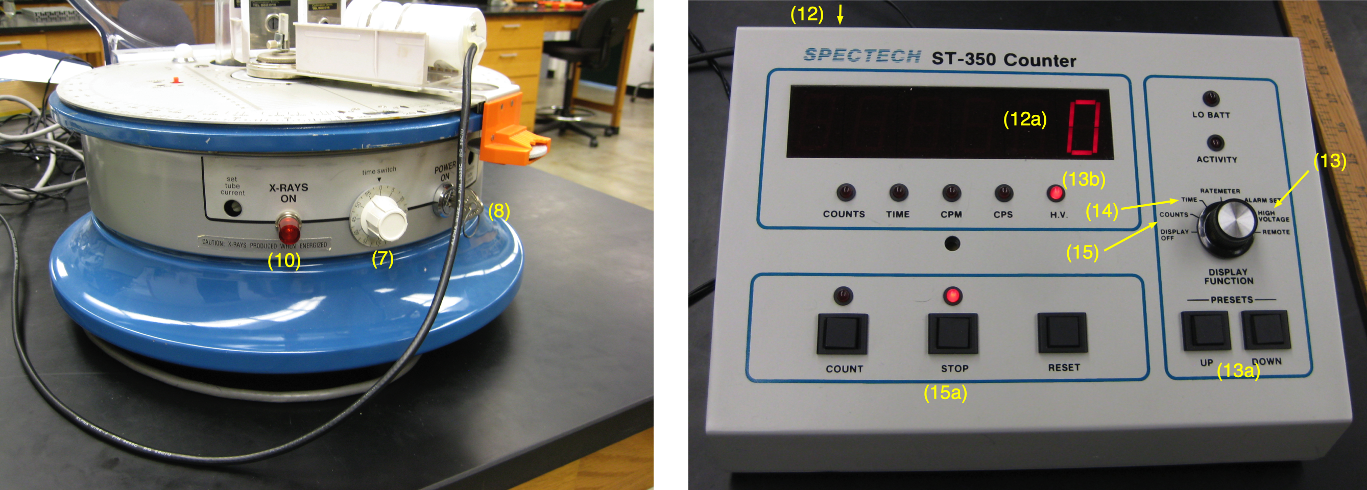
Fig. 27.4 The main controls of the X-ray apparatus(left) and the readout electronics (right).

The apparatus is shown in Fig. 27.3 Study it carefully making sure you can identify the various features. The plastic cover (1), which absorbs scattered radiation, is opened by sliding it sideways (parallel to the hinges (1a)) about half an inch either way from its central position. Note that the cover must be closed and in the central position before high voltage may be applied to the X-ray tube.

The 1 mm vertical slit (TEL 582.001, (c1)) should be attached to the X-ray tube window (2). Similarly the 3 mm vertical slit (TEL562.016, (c2)) should be placed in slot number 13 on the slide carriage and the 1 mm slit (TEL562.015, (c3)) in slot number 18. The Geiger-Muller tube holder should be placed with the locating plates in slots 22 and 26 (3). Swing the slide carriage slowly around until the cursor gives an accurate zero reading on the \(2\theta\) (4) scale Check that the \(\theta\) scale (4a) also reads zero. Check that the crystal post (5) rotates through half the angle that the slide carriage rotates.

Using tweezers, remove the NaCl crystal (5a) from its vial and mount it on the crystal post. Do not touch the crystal with your fingers and do not over-tighten the clamp, as the crystal is very fragile.

Check that the voltage selector switch (6) is set at 30 kV. Move the slide carriage counter-clockwise from the \(0^o\) position to an angle of at least \(20^o\), then close and center the plastic cover (1). Turn the timer switch (Fig. 27.4 (7)) to 55 minutes then turn on the main power using the key (Fig. 27.4 (8)) on the control panel. At this stage both the white POWER ON lamp (9) and the X-ray tube filament(9a) should be illuminated. Wait a few minutes then press the red ON button (Fig. 27.4 (10)). The red lamp (11) should now be illuminated indicating that the X-ray tube is functioning. If a faint crackling sound is heard, turn off the X-rays by sliding the plastic cover sideways. Wait a few more minutes and try again.

The X-ray photons are detected using a Geiger-Mueller (GM) tube which is basically a charged, cylindrical capacitor. An incoming photon ionizes the gas in the capacitor and leads to a discharge producing a small current pulse that can be detected electronically. The count rate (counts/second) is a measure of the X-ray intensity

Connect the coaxial cable to the counter (12). Set the GM tube voltage to 400 - 420 V by setting the function switch to HIGH VOLTAGE (13) and using the UP and DOWN buttons (13a). The current value of the high voltage is shown in the display (12a) (the row of LED’s (13a) indicates the quantity currently being shown in the display).

You can get a first impression of the variation of the X-ray intensity with angle by setting the function switch to RATEMETER and using the UP and/or DOWN buttons to select CPS (Counts Per Second) in the display. Once you start counting by pressing the COUNT button (15a) the display will show the number of counts per second.

This number will fluctuate due to the random nature of the X-ray emission process. Starting at \(2\theta = 20^o\), slowly increase the angle and observe how the rate changes. This should give you an impression where the largest variations in intensity are located. The next step is a systematic study of the intensity as a function of the angle \(2\theta =.\)

Set the function switch on TIME (14) and set it to 10 seconds using the UP and DOWN buttons (13a) and the display (12a). In order to take data set the function switch to COUNTS (15). You start the counter by pressing the COUNT button (15a), counting should stop automatically after 10 seconds (or whatever value you set it to in the previous step) To clear the counter value, press the RESET button.

Starting again at \(2\theta = 20^o\), record 10 second counts at \(1^o\) intervals up to \(120^o\). Where the count rate appears to peak, reduce the interval to 10’. To do this use the thumb wheel scale. The thumb wheel (10) operates through a friction drive and may be reset as follows. Set the cursor to the nearest whole degree mark to the center of the peak. Holding the slide carriage firmly in place, rotate the thumb wheel against the friction drive until you obtain a zero setting. Release the slide carriage and double-check that your adjustment is precise. You may now backtrack to cover the peak at the required 10’ intervals. When your measurements are complete, return the crystal to its vial.

27.3.1. Analysis

1. Plot a graph of counts (y-axis) vs. angle \(2\theta\) (x-axis) including error bars in the counts (\(\sigma_N = \sqrt(N)\), where \(N\) are the counts). Hint: you can combine two numpy arrays into one (e.g. coarse_angles data and fine_angles) by doing:

   all_angles = np.append(coarse_angles,fine_angles)
   

2. Identify on the graph the K\(\alpha\) and K\(\beta\) peaks and the order, \(n\).

3. Determine the peak positions and their uncertainties and document how you determined or estimated your position uncertainties. (for helpful tools, see Collection of useful tools)

4. For each X-ray line make a plot of \(sin(\theta)\) (y_axis) as a function of \(n\), make sure you estimate your error in \(sin(\theta)\) using error propagation.

5. Fit a line through the points of each X-ray line and determine the spacing \(D\) from the slope. Determine the average value for the spacing \(D\) and its error.