28. Normal Zeeman Effect

28.1. Background

Due to the orbital motion and spin of atomic electrons, an atom possesses a magnetic dipole moment. In an external magnetic field, the total energy of the atom now includes magnetic potential energy that is dependent on the orientation of the dipole moment in the external field. Since this orientation is quantized (“space quantization”), so too is the potential energy. Spectral lines, which correspond to transitions between states of different total energy associated with these atoms are now being split into a number of very closely spaced lines when the atoms are in a magnetic field (Fig. 28.1).

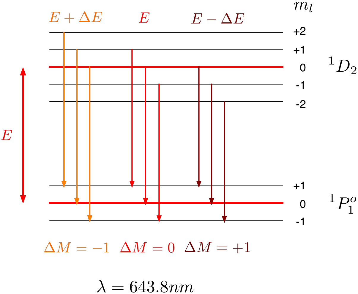
Fig. 28.1 Schematic of the energy levels and transitions leading the the red Cd line. Without magnetic field all levels with different \(m_l\) values would have the same energy (indicated by the red horizontal lines).

The normal Zeeman effect is exhibited in transitions between states characterized by a total spin of zero, where the magnetic moment is solely due to the orbital motion of the electrons. The red 643.8 nm cadmium line falls into this category. It is due to the transition between a \(^1D_2\) and a \(^1P_1\) (\(^{2S+1}L_J\)) state. In an external magnetic field, \(\vec{B}\), the line is split into three lines. The emitted photons have energies \(E- \Delta E\) , \(E\), and \(E+ \Delta E\), where \(E\) is the energy with no magnetic field present and

(28.1)\[\Delta E = \mu_B |\vec{B}|\]

where \(\mu_B = \frac{e\hbar}{2m}\) is the “Bohr magneton”. It has a value of \(9.27\times 10^{-24}\) J/T and will be determined from this experiment. The problem is that even for a field of \(1\ T\), \(\Delta E\) is very small. You can estimate the fractional change in the wavelength to be

(28.2)\[f_l = \Delta\lambda/\lambda= \frac{\lambda}{hc}\Delta E \approx 3\times 10^{-5}\]

This small value of \(\Delta \lambda\) can be measured with a Fabry-Perot interferometer, which is a so-called multiple beam interferometer. The principle is shown in Fig. 28.2.

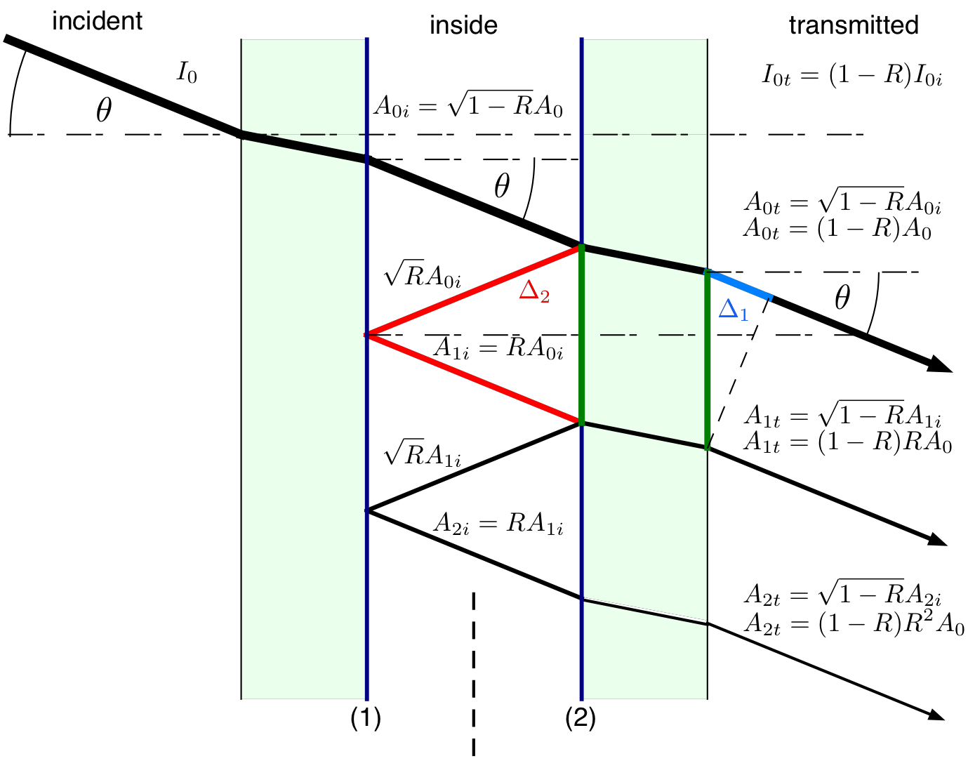
Fig. 28.2 Light passage in a Fabry-Perot interferometer.

An incident ray of intensity \(I_0\) and amplitude \(A_0\) is incident on 2 glass planes which have partially reflective surfaces ((1) and (2) in Fig. 28.2). Each surface has a reflectivity \(R\) and a transparency \(T = 1 - R\). The intensity of the incident beam in between the reflective surfaces is \(I_{i0} = (1-R)I_0\) and the amplitude of the EM wave correspondingly is \(A_{i0} = \sqrt{1-R}A_0\). Part of this wave is reflected back at the surface (2) and again at surface (1) after which it is again incident of surface (2) with a reduced amplitude \(A_{i1} = RA_{i0}\) (at each reflection the amplitude is reduced by a factor \(\sqrt(R)\)). From the first beam the amplitude of the transmitted wave is \(A_{0t} = \sqrt{1-R}A_{0i} = (1-R)A_0\). From the second beam the amplitude of the transmitted wave is \(A_{1t} = \sqrt{1-R}A_{i1} = (1-R)RA_0\). These two waves and all the additional transmitted waves with amplitudes \(A_{nt} = (1-R)R^n A_0\) will interfere. To calculate the total amplitude, the path length differences between the waves need to be calculated. The path length difference between \(A_{0t}\) and \(A_{1t}\) is \(\Delta_2 - \Delta_1\) (see Fig. 28.2) with:

(28.3)\[ \begin{align}\begin{aligned}\Delta_1 = 2d \tan{(\theta)} \sin{(\theta)}\\\Delta_2 = \frac{2d}{\cos{(\theta)}}\\\delta = k (\Delta_2 - \Delta_1) = k2d \cos{(\theta)}\end{aligned}\end{align} \]

The angle \(\delta\) is the phase shift between the two rays. Each subsequently transmitted has this phase shift with respect the previous one. Using complex numbers to express the amplitude one obtains for the \(n^{th}\) transmitted wave including the phase shift with respect to \(A_0\)

(28.4)\[A_n = (1-R) R^n e^{i n \delta} A_0\]

Assuming that the two mirrors are infinitely large, one obtains an infinite number of reflections and consequently the total amplitude will be:

(28.5)\[ \begin{align}\begin{aligned}A_{tot} = (1-R) (\sum_{n=0}^\infty{ (R e^{i\delta})^n} ) A_0\\A_{tot} = (1-R) A_0 \frac{1}{1-Re^{i\delta}}\end{aligned}\end{align} \]

To obtain the intensity one needs to calculate:

(28.6)\[I_{tot} = A_{tot}A_{tot}^* = I_0 \frac{(1-R)^2}{1+R^2 - 2R\cos{(\delta)}}\]

The intensity has a maximum when \(\cos{(\delta)} = 1\) which means that \(\delta = m 2\pi\) which is equivalent to

(28.7)\[2d \cos{(\theta)} = m \lambda`.\]

As a consequence \(\theta\) decreases with increasing \(m\) for constant \(\lambda\). For the red Cd line and a typical mirror separation of \(d = 1\)mm the intensity as a function of \(\theta\) and for two values of reflectivities is shown in Fig. 28.3.

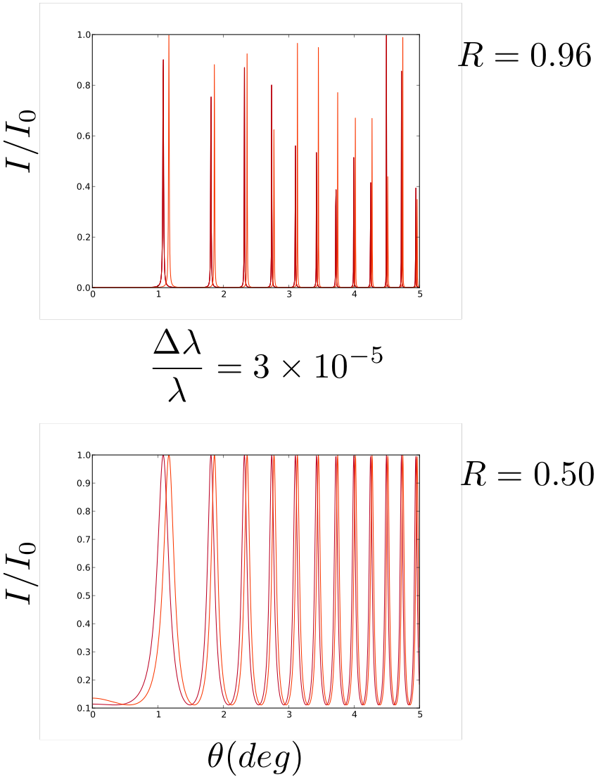
Fig. 28.3 Angular distribution of the transmitted intensity of the red Cadmium line. Top: for a reflectivity R=0.96. Bottom: R = 0.5. The two sets of lines correspond to two wavelengths with \(\Delta\lambda/\lambda = 3\times 10^{-5}\).

You can clearly see that the larger reflectivity leads to a better separation of the two wavelengths.

28.2. Experimental Procedure

The apparatus is shown schematically in Fig. 28.4. A Cadmium lamp is placed between the poles of an electromagnet. Light emitted by th lamp passes through a Fabry-Pero (FP) etalon. A red filter is used to isolate the red Cadmium line. The circular fringes produced at infinity by constructive interference are imaged as circular rings in the focal plane of the telecopy lens (\(f = 183\ mm\)). This intermediate image can either be viewed using an eyepiece or it is viewed by a CCD camera. In order to be able to take and analyze data you need to perform the following tasks:

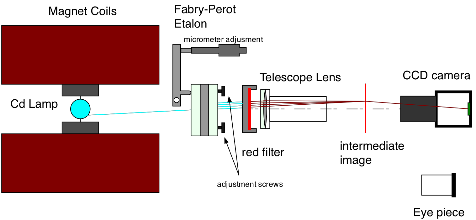
Fig. 28.4 Schematic of the experimental setup.

1. Determine the magnetic field at the location of the lamp for a given coil current.

2. Align the Fabry-Pero etalon by CAREFULLY using the alignment screws. The FP-etalon is extremely sensitive. You can easily see small vibrations of the table.

3. Calibrate the CCD camera.

28.2.1. 1. Magnetic Field Measurement

Unscrew the cadmium lamp from its holder. Turn on the cooling water supply for the electromagnet. Switch on the magnet power supply and gradually increase the current to 10.0 A. Use the gauss-meter to measure the magnetic induction, B (T), halfway between the poles. The correct value is the maximum value, obtained when the plane of the probe is held perpendicularly to the field. Decrease the current to zero and switch off the power supply. Replace the cadmium lamp, being careful not to alter the gap between the poles, and switch the lamp on (0.9 A). The Cadmium lamp takes about 5 - 10 min to fully warm up.

28.2.2. 2. Aligning the FP Etalon and Data Taking

Align the axis of the interferometer with the cadmium lamp. Without the red filter or telescope in place, turn the adjusting screws on the nearer partially reflecting plate until circular fringes are seen. You can also use the large micrometer screw to adjust the overall distance \(d\) between the plates. Note: whenever you change the alignment screws \(d\) varies as well. Make only small correction and try to obtain the sharpest fringes possible. Replace the telescope objective. Look into the telescope without camera or eyepiece and make sure you still see the fringes. Make more adjustments to get the best result. Align the camera with the telescope and the lamp. Start the camera control program on the computer and open a life view with about 10 frames per second. The distance between the end of the telescope lens and the camera lens should be about 11 cm. Adjust the focus of the camera to get a sharp image of the fringes. Every time you adjust the alignment you should also adjust the focusing. Once you have the sharpest fringes you can carefully place the red filter on the telescope lens. DO NOT TOUCH THE ALIGNMENT SCREWS when you are doing this or you have to re-adjust them again. Try to further optimize the sharpness the red fringes. In the end they should look like those in Fig. 28.5.

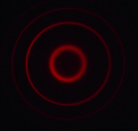
Fig. 28.5 Fringes (with red filter) of the red Cadmium line without magnetic field.

Take a picture of your sharp fringes and save it to disk. Now you are ready to turn on the magnetic field. Do this SLOWLY ! Once you reach 10A you should see that each fringe has spit up in several fringes (as an example see Fig. 28.6). You can still try to optimize the sharpness of the fringes. Once you have a good picture take snap-shots with the camera. You will see that the quality of the images continually changes slightly. Be patient! Once you have taken a few good images turn off the magnetic field.

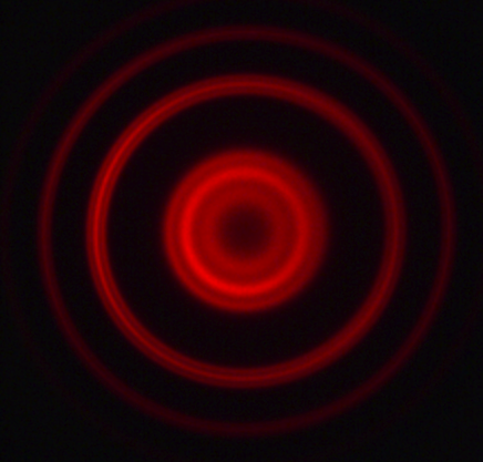
Fig. 28.6 Fringes with magnetic field.

28.2.3. 3. Camera Calibration

Now it is time to take a calibration image with the current setting (focus) of your camera. It is important that you DO NOT CHANGE ANYTHING on the camera after you took pictures from the fringes. Take the small caliper and place it before the camera such that you see a sharp image. Record the image. Now you have your calibration and you are ready to analyze the images. A typical calibration picture us shown in Fig. 28.7

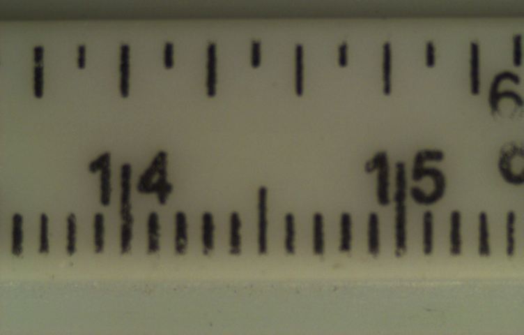
Fig. 28.7 Picture of a ruler to calibrate the camera.

28.3. Data Analysis

From the diameters of adjacent rings (without magnetic field) determine the order \(m\) and the spacing \(d\) between the plates. From the splitting of the lines, determine \(\Delta \lambda\) and therefore \(\Delta E\) and with the the knowledge of \(|\vec{B}|\) you can determine \(\mu_B\), Bohr’s magneton.

28.3.1. Determining \(\frac{\Delta \lambda}{\lambda}\)

The geometry of image formation by the telescope lens is shown in Fig. 28.8.

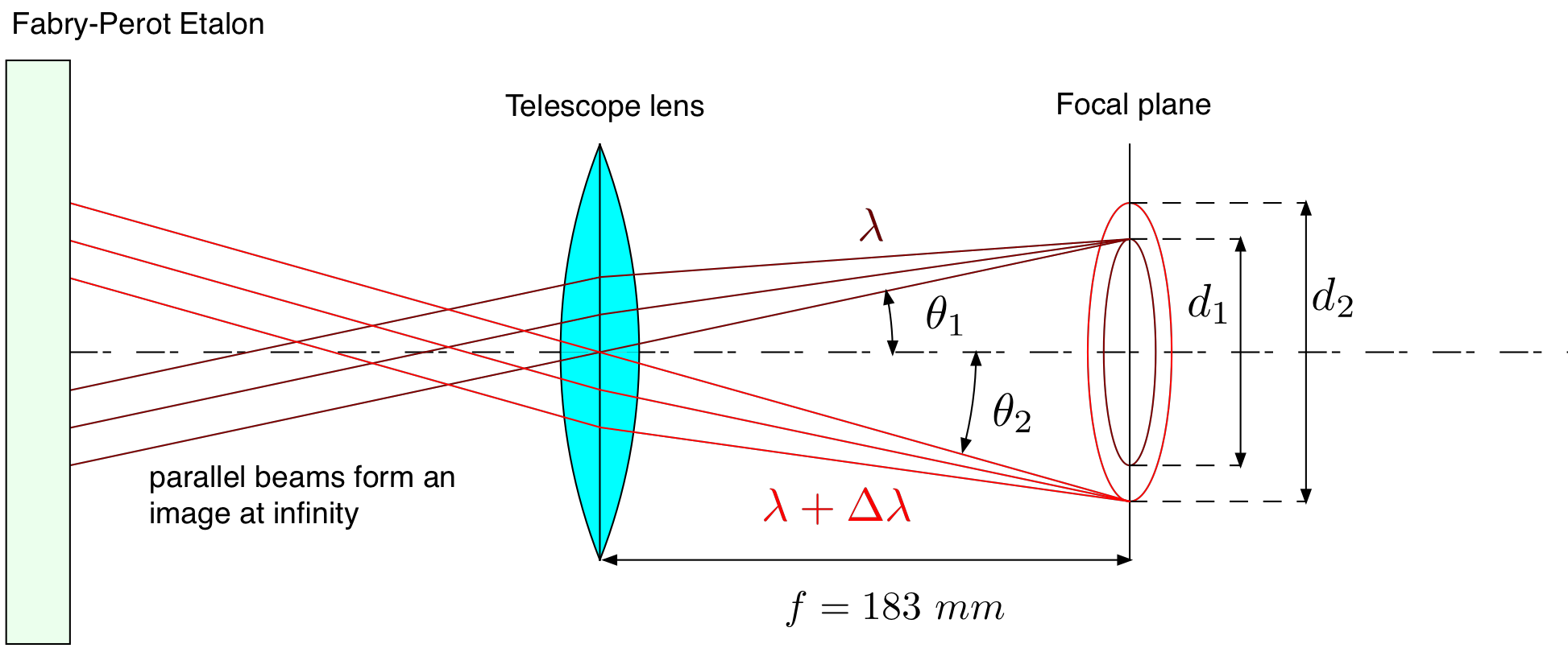
Fig. 28.8 Image formation of fringes in the focal plane of the telescope lens.

Parallel beams of light with a wavelength \(\lambda\) make an angle \(\theta_1\) with respect to the optical axis of the telescope lens and are focused on a ring in the focal plane with a diameter \(d_1\). Parallel beams with a different wavelength \(\lambda + \Delta \lambda\) make an angle \(\theta_2\) and are focused on a ring with diameter \(d_2\). These angles are determined by the relation (28.7). The following geometric relations hold:

(28.8)\[ \begin{align}\begin{aligned}d_1 = 2f \tan{(\theta_1)}\\d_2 = 2f \tan{(\theta_2)}\\d_1^2 = 4f^2 \frac{1-\cos{(\theta_1)}^2}{\cos{(\theta_1)}^2}\\d_2^2 = 4f^2 \frac{1-\cos{(\theta_2)}^2}{\cos{(\theta_2)}^2}\end{aligned}\end{align} \]

using \(cos{(\theta_1)} = \frac{m\lambda}{2d}\) and \(cos{(\theta_2)} = \frac{m(\lambda + \Delta \lambda)}{2d}\), together with the approximations \((\lambda + \Delta \lambda)^2 \approx \lambda^2 + 2\lambda\Delta\lambda\) and \(1+2\frac{\Delta\lambda}{\lambda}\approx 1\) one obtains:

(28.9)\[ \begin{align}\begin{aligned}\frac{d_2^2}{4f^2} - \frac{d_1^2}{4f^2} = -2\frac{\Delta\lambda}{\lambda}\\\frac{\Delta\lambda}{\lambda} = \frac{d_1^2 - d_2^2}{8f^2}\end{aligned}\end{align} \]

which is independent of the order m.