21. Compton Scattering with Scintillation Detector

21.1. Background

When a photon is scattered by a charged particle, such as an electron, it imparts some of its energy and momentum to the particle, which then recoils. The photon comes away from the collision with less energy and therefore longer wavelength than it had before the collision. In 1922, Compton applied the laws of conservation of energy and momentum to a collision between a photon and a free electron to obtain an expression for the change in wavelength as a function of the scattering angle, \(\theta\) , the photon Fig. 21.1:

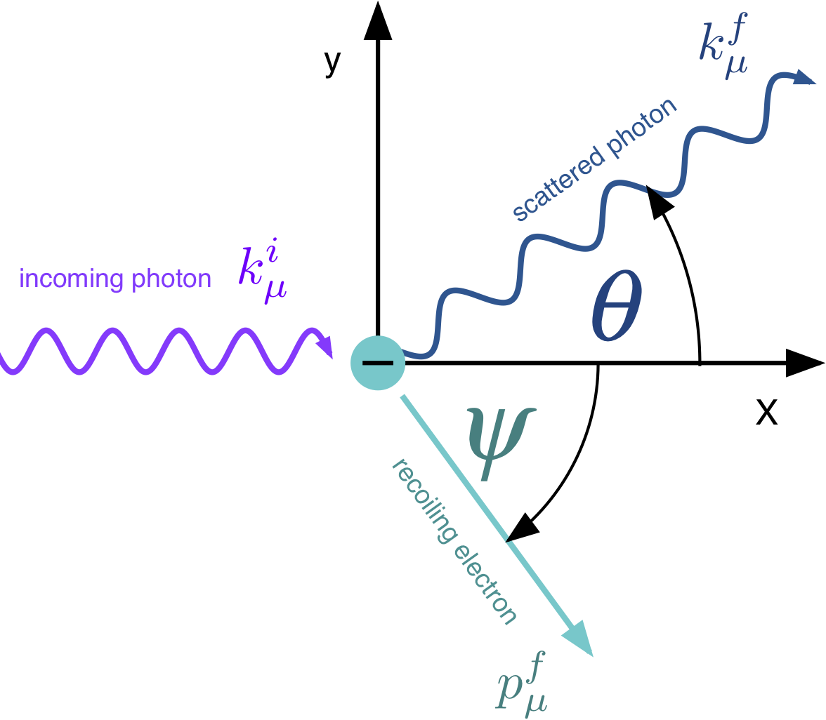
Fig. 21.1 Compton scattering of a photon off a charged particle.

Here

\[\begin{split}k_\mu ^i = \left( {\begin{array}{*{20}{c}} {{{\vec k}_i}} \\ {{E_0}} \end{array}} \right),\left| {{{\vec k}_i}} \right| = {E_0}\end{split}\]

is the 4-vector of the incoming photon (\(\vec{k}\) is the photon momentum and \(E_0\) the photon energy),

\[\begin{split}k_\mu ^f = \left( {\begin{array}{*{20}{c}} {{{\vec k}_f}} \\ {{E_f}} \end{array}} \right),\left| {{{\vec k}_f}} \right| = {E_f}\end{split}\]

is the 4-vector of the scattered photon and

\[\begin{split}p_\mu ^f = \left( {\begin{array}{*{20}{c}} {{{\vec p}_f}} \\ {{E_R}} \end{array}} \right),{E_R} = \sqrt {p_f^2 + {M^2}}\end{split}\]

is the 4-vector of the recoiling particle (\(\vec{p_f}\) is the momentum of the recoiling electron and \(E_R\) its total energy).

The 4-vector of the electron at rest is

\[\begin{split}p_\mu ^i = \left( {\begin{array}{*{20}{c}} {{0}} \\ {{M}} \end{array}} \right)\end{split}\]

Note that natural units are used where \(c = 1\)

Energy conservation leads to the following expression:

(21.1)\[{E_0} + M = {E_f} + \sqrt {p_f^2 + {M^2}}\]

and momentum conservation :

(21.2)\[\begin{split}\begin{array}{*{20}{c}} {{E_0} = {E_f}\cos (\theta ) + {p_f}\cos (\psi )} \\ {0 = {E_f}\sin (\theta ) - {p_f}\sin (\psi )} \end{array}\end{split}\]

From equations (21.1) and (21.2) one can solve for \(E_f\) as a function of \(\theta\) and obtains:

(21.3)\[{E_f} = \frac{{{E_0}}}{{1 + \frac{{{E_0}}}{M}\left( {1 - \cos (\theta )} \right)}}\]

Using the relation \(E = \frac{{hc}}{\lambda }\) equation can be used to calculate the change in wavelength of the photon leading to:

(21.4)\[\Delta \lambda = {\lambda _f} - {\lambda _i} = \frac{h}{{mc}}\left( {1 - \cos (\theta )} \right)\]

The expression \(\frac{h}{mc}\) is called the Compton wavelength.

21.2. Experimental Setup

Fig. 21.2 Compton scattering experimental setup.

Fig. 21.2 shows your experimental setup. The source is strong ¹³⁷Cs source that is housed in a lead cylinder with an opening that you instructor needs to open and close. Target is an aluminum cylinder which can be removed. The detector is a NaI(Tl) scintillation detector that you probably have used previously and should be setup as described in the Scintillator experiment. Close to the target is an angle scale where you can read and set the scattering angle.

The goal of this experiment is to measure the energy of the scattered photons as a function of their scattering angle, to verify the expression from equation and to determine the mass of the recoiling particle.

21.3. High Energy Photon Detection

21.3.1. Scintillation Materials

The detection of ionizing radiation by the scintillation light produced in certain materials is one of the oldest techniques on record. In Geiger and Marsden’s famous scattering experiment of \(\alpha\) particles off Gold nuclei, the scattered \(\alpha\) particles were observed via the scintillation light they produced when they hit a ZnS-screen. ZnS produced light flashes, called scintillation light, when hit by an \(\alpha\)particle. The scintillation process remains one of the most useful methods available for the detection and spectroscopy of a wide assortment of radiation.

The scintillation material used in this experiment is NaI(Tl) where (Tl) means that there are small mounts of Tl (Thallium) mixed into the NaI. Scintillation light is produced when a fast, charged particle excites the electrons in the NaI crystal from their valence band into the conduction band and leaving a hole in the valence band. The Thallium impurity in NaI produces so-called activator centers, which allow the electrons and the holes to recombine quickly with the emission of visible light. This light is detected by a photo-multiplier (Fig. 21.3) that produces an electrical current pulse proportional to the number of photons observed. A good scintillator should convert the kinetic energy of the charged particle in to visible light efficiently and linearly. The decay time of the light should be fast so that fast pulses can be generated and high particle rates can be measured.

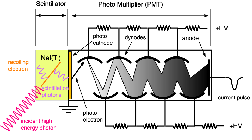
Fig. 21.3 Schematic of scintillator and photo multiplier (PMT)

21.3.2. Photo Multiplier

The photomultiplier is an instrument that can detect photons. An incoming photon (e.g. a scintillation photon) hits the photo-cathode and via photo effect releases an electron. The probability for this process is about 20%, so you need on the average 5 photons to produce a single photo-electron. The released electron is then accelerated toward a metal plate called a dynode where upon impact it releases more electrons, typically 2. These in turn are accelerated to the next dynode where each electron knocks out 2 more electrons. In this matter one obtains an exponentially growing number of electrons. At the end all the released electrons are collected at the Anode where they produce a short, measurable electric current pulse.

21.3.3. Electronics and Data Acquisition

The output pulses of the PMT are amplified and then recorded. The size of a pulse is proportional to the number of photons hitting the photocathode. These in turn are proportional to the amount of energy the charged particle deposited in the scintillator. Therefore the output pulse is proportional to the energy deposited in the scintillator. The proportionality constant has to be determined experimentally. This process is called calibrating the detection system.

The amplified pulses are analyzed by an Analog to Digital Converter (ADC) which determines the pulse height and converts it into a number (typically between 0 and 1023, or 0 to 2047). These (ADC) numbers are then histogrammed i.e. each possible ADC value has a counter associated with it and each time a certain value occurs the corresponding counter is incremented. So if your ADC has a range from 0 to 1023, you have a total of 1024 counters. Each ADC value is called a channel and the counter value is called the channel contents. If you take data for a while you will see that some values occur more frequently than others. The total set of counter values and the corresponding ADC values is called a spectrum. When you plot a histogram the x-axis corresponds to the ADC value and the y-axis represents the corresponding counter values or channel contents. The process described above is performed by a Multi Channel Analyzer (MCA). The hardware part is installed in a PC and the associated software (Maestro) is running on the computer. A schematic of the setup os shown in Fig. 21.4

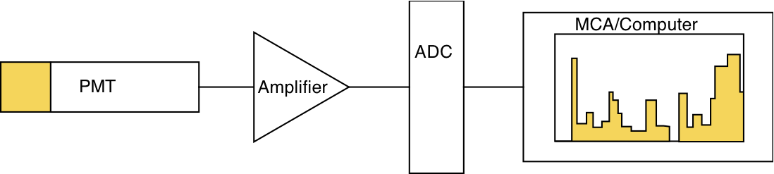
Fig. 21.4 Schematic of the data acquisition with PC.

21.3.4. Detection of Photons

A scintillator is primarily sensitive to the passage of charged particles. High energy photons, like all photons, are not charged and can only be observed if they produce a fast moving charged particle which subsequently interacts with the scintillator material. The energy that is measured in a scintillator is therefore the energy deposited by charged particles, mostly electrons, that interacted with the incoming high energy photon. The main reactions between a photon and the electrons in the scintillator are:

• Photo effect:: a photon is absorbed by an electron which then interacts with the crystal. \(K_e = E_\gamma - B_e\) , where \(K_e\) is the kinetic energy of the electron, \(E_\gamma\) is the photon energy and \(B_e\) is the electron’s binding energy.

• Compton scattering: a photon scatters off an atomic electron, the electron recoils and has kinetic energy, the original photon changes direction and loses energy corresponding to the recoil energy of the electron. \(M_e\) is the mass of the electron and the energy of the recoiling electron is given by \(K_e = E_\gamma - E_f\) while energy of the scattered photon is given by

(21.5)\[{E_f} = \frac{{{E_\gamma}}}{{1 + \frac{{{E_\gamma}}}{M_e}\left( {1 - \cos (\theta )} \right)}}\]

• Pair production: a photon (with a an energy > 1.2 MeV) converts into an electron – positron (anti-electron) pair. The electron is stopped in the crystal, the positron eventually annihilates with an atomic electron and produces two 0.511 MeV photons which may or may not be detected.

• Rayleigh scattering: a photon scatters off an atom without excitation. This does not produce a measurable effect in the scintillator

The probability of each of these process depends on the photon energy and the composition of the scintillator material. From all the processes which produce signals in the detector (those highlighted above) the most important one for the source we are using is Compton scattering. This can be seen from studying the cross sections for these processes for Carbon and Lead in the following figure. Note that this is a log-log plot! For Carbon, Compton scattering is dominant for photon energies between about 100KeV and 10 MeV while for Lead the photo electric process dominates up to about 700KeV when Compton scattering starts to dominate.

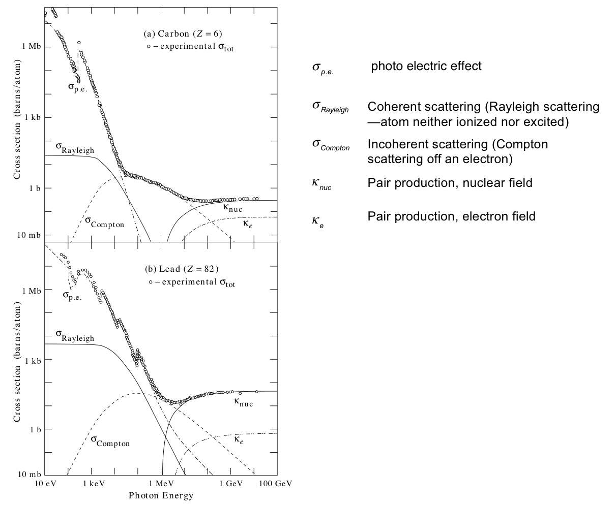
Fig. 21.5 Cross sections for the various processes occurring in a scintillator.

In order to use a scintillation detector one has to understand the spectrum produced by a scintillator when a high energy photon interacts with it. You should always remember that several of the processes listed above can occur sequentially with a single initial photon and that it is the total energy of the recoiling electrons that is measured in this process. If mono energetic photons enter the scintillator and transfer all their energy to the electrons which all get stopped in the scintillator then the signals at the end of the PMT should all have basically the same value. This means that the histogram should show a peak. If a Compton scattered photon leaves the scintillator without further interaction then the maximum energy deposited in Compton scattering would correspond to a photon scattering angle of 180 degrees. A schematic spectrum of a scintillator measuring photons with the same energy and where \(E_\gamma \leq 1 MeV\) would look like (Fig. 21.6):

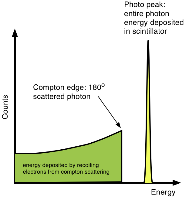
Fig. 21.6 Schematic of a scintillator spectrum of mono energetic photons.

21.3.5. PMT Operation

The photo multiplier requires high voltage (HV) in order to accelerate the secondary electrons to the anode. It is supplied by the Ortec 556 module. Before you turn it on, make sure the knobs are set to 0. Turn the unit on and then set it to 700-800V. The output of the PMT should be connected to the input of the Ortec 590A amplifier. Connect the output of the amplifier with a BNC ”T” to an Oscilloscope and continue the connection to the input of the ADC. Place a 137Cs source on the scintillator and check if you see pulses on the oscilloscope. Make sure the signals are in the range of 2 – 5 V. What you see is the histogram (spectrum) of pulses described previously.

21.3.6. Decay Schemes of \(^{137}Cs\) and \(^{60}Co\)

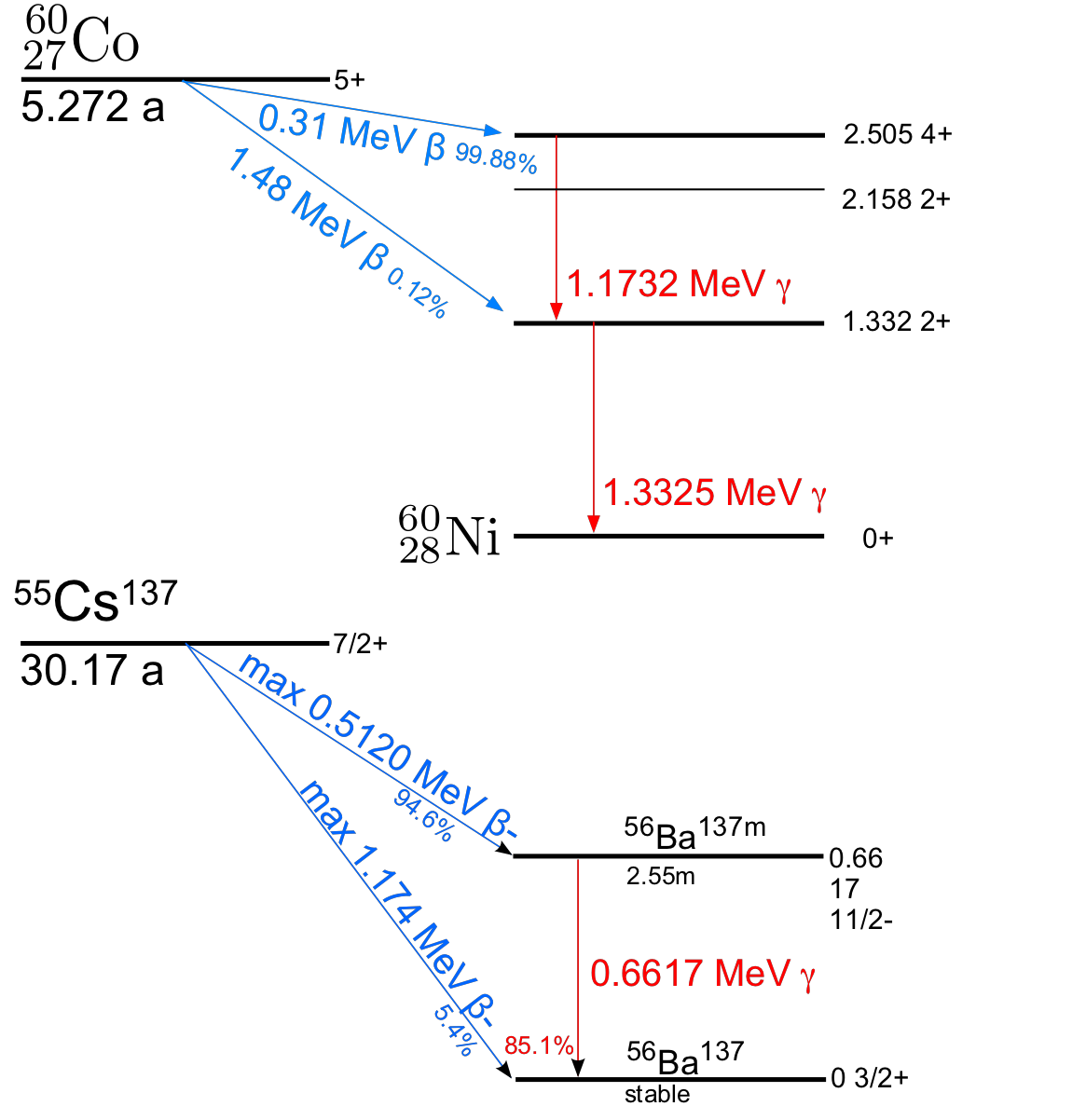
Fig. 21.7 Decay schemes and photon energies.

The red arrows indicate the photons to be detected by the NaI(Tl) scintillator. The photons are emitted when the excited daughter nuclei transition into their ground states. The exited daughter nuclei are the result of a beta decay of the parent nuclei. Using the photo peak of these two sources calibrate the spectra such that instead of channels (or bin numbers) you have KeV or MeV. M

21.4. Pre-Lab Preparation

From LabTools review working with MCA data and energy calibration

You need to be able to answer the following questions:

• What is Compton Scattering?

• What is the Photo Effect?

• What is a scintillator?

• How to you load a MCA spectrum

• What is the typical energy of a visible light photon?

• How do you carry out an energy calibration?

• How do you determine a peak position by fitting?

21.5. Experimental Procedure

21.5.1. Taking Data

1. Set the MCA live time to 300s. Set the detector at 0 degree and remove the target. Push the scintillator towards the target (this should not require any force) in such a way that about 1 inch sticks out of the surrounding lead ring. Place a ⁶⁰Co source on the detector and take a spectrum. This spectrum will show a very prominent peak for ¹³⁷Cs and the two peaks of ⁶⁰Co. You will use this spectrum to calibrate the instrument. Make sure that you select to save an ASCII spectrum with the extension. Do not change anything in the detector electronics once you measured the calibration spectrum. Now you are ready to take your data.

2. Start at and angle of 20 degrees and take a spectrum with and without target. At this angle I would recommend you accumulate events for 4 minutes. Make sure that you select to save an ASCII spectrum with the extension.

3. Continue this procedure in steps of 20 degrees until you have reached 120 degrees. See Section 21.5.2

Remember : save all the spectra as SPE (ASCII) files. In that way you can analyze them later using the LabTools and working with MCA data package.

21.5.2. Recommended Acquisition Times:

Scattering Angle	Time (in minutes)
30	5
40	5
60	10
80	10
100	10
120	10

21.6. Analysis

• Finish the derivation of equation (21.3)!

• Load your calibration spectrum to determine the energy calibration (Look at the documentation working with MCA data).

• Check in Collection of useful tools for Python code examples that are helpful for your analysis e.g. selecting data and peak fitting.

• From the combined measured \(^{137}Cs\) and \(^{60}Co\) spectrum, determine the position (in channel numbers) of the photo peaks.

• Fit (use linefit) the known values of the photon energies (see Fig. 21.7) as a function of channel numbers to determine the calibration function to convert channel numbers to energies.

• Make a plot of the calibration points and the fitted line.

• Make a plot of the calibrated spectrum and indicate the energies of the photo-peaks used in the calibration.

• Apply the calibration function to all spectra taken.

• From all spectra taken with the target subtract the corresponding spectrum taken without a target. Make sure that both spectra have been taken with the same lifetime, other wise correct for the lifetime before you take the difference. This leaves you with an energy spectrum of the scattered photons only.

• Determine the energy of the photo peak (fit a Gaussian to the photo peak). This gives you the energy of the scattered photons.

• In order to verify that equation (21.3) holds, plot the ratio \(\frac{E_0}{E_f}\) versus \((1-cos(\theta))\). Then fit a line through the data.

• Check the offset and the slope. From the slope you can determine the mass of the recoiling particle. If the photons scatter of electrons then this should be the electron mass. How close are you ?