20. Rutherford Scattering

Today’s understanding of the atom, as a structure whose positive charge and majority of mass are concentrated in a minute nucleus, is due to the \(\alpha\)-particle scattering experiments conducted by Ernest Rutherford and his colleagues (1909-1914). The essential features of Rutherford’s apparatus are shown in Fig. 20.1: \(\alpha\)-particle emitted from a radioactive source strike a thin gold foil. Most pass straight through the foil, but a fraction are scattered at an angle \(\theta\) into the detector. The smaller the distance of closest approach between an \(\alpha\)-particle and a gold nucleus, the larger is the scattering angle.

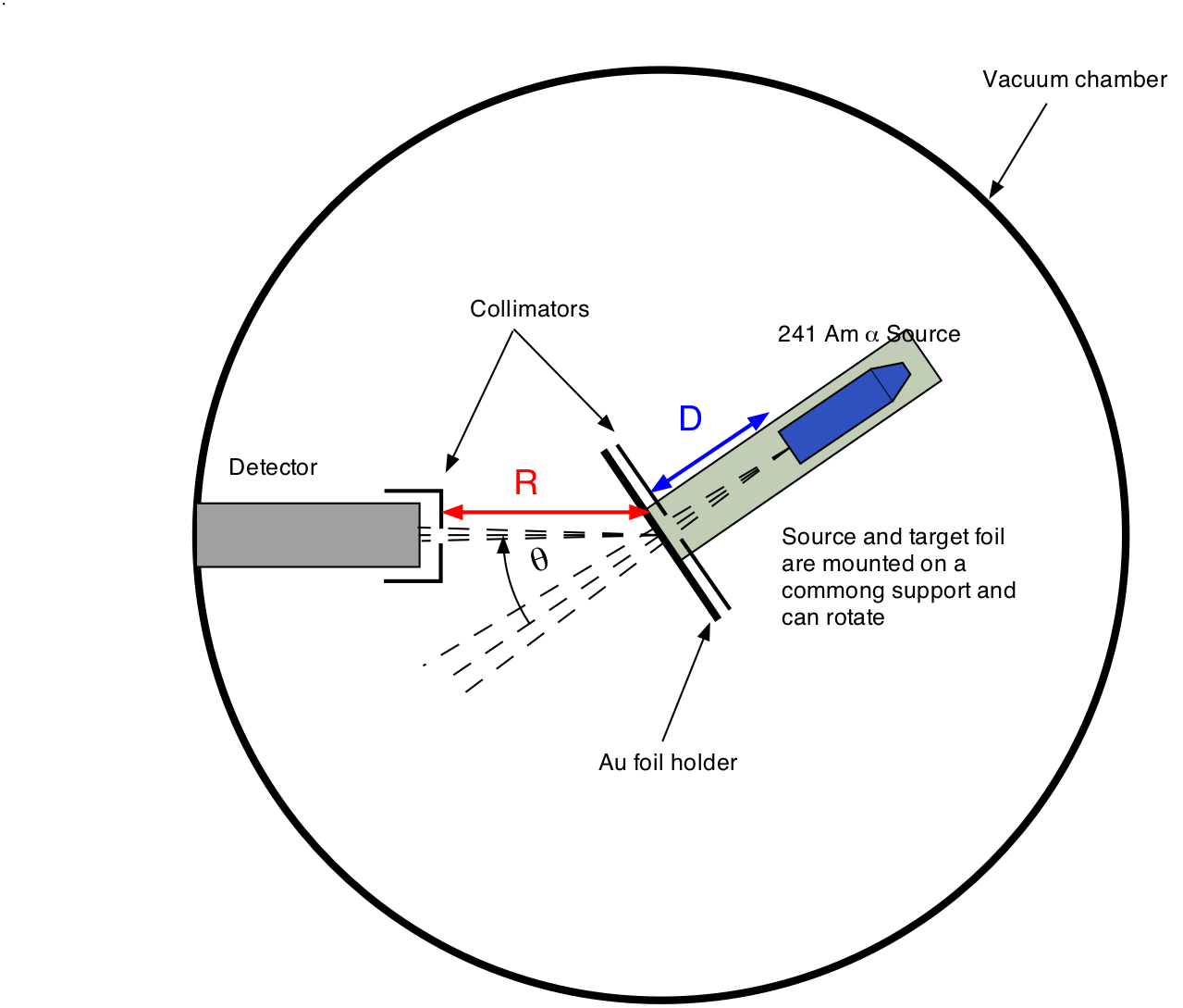
Fig. 20.1 Setup for \(\alpha\)-particle scattering off Gold

20.1. Background Information

A theoretical analysis of the scattering process under the assumption of the existence of a small massive nucleus leads to the following expression for the cross section:

(20.1)\[\frac{d\sigma }{d\Omega} = \frac{\left( zZe^2\right)^2} {\left( 4\pi \varepsilon_0 \right)^2 \left( 4E_{kin}\right)^2} \frac{1}{\sin^4 \left(\theta /2 \right)}\]

where \(z\) is the charge of the projectile (for an \(\alpha\)-particle \(z = 2\)) and \(Z\) is the charge of the nucleus (for Au \(Z = 79\)), \(E_{kin}\) is the kinetic energy of the projectile (for ²⁴¹Am the \(\alpha\)-particle has an energy of 5.486 MeV) and \(\theta\) is the scattering angle. The quantity \(\frac{{d\sigma }}{{d\Omega }}\) is the differential cross section and \(d\Omega\) is the solid angle. The geometric interpretation of the cross section and solid angle are shown in Fig. 20.2.

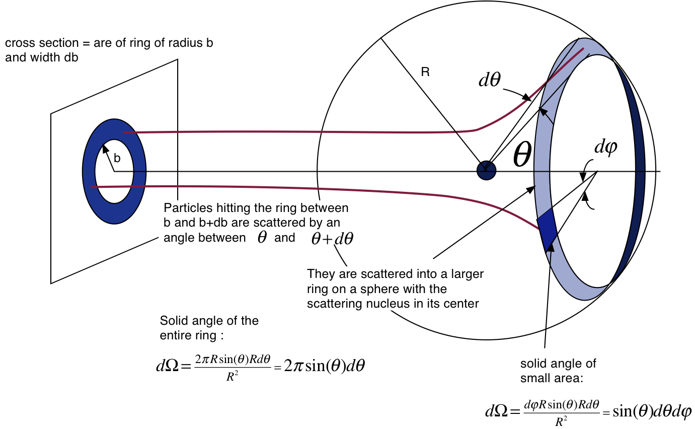
Fig. 20.2 Geometry of the cross section and the solid angle

The cross section given in equation (20.1) is for one nucleus only. In order to calculate the rate at which particles are scattered at a certain angle one needs to know the flux of the incoming particles \(\vec{j} = \frac{{\dot N}_{inc}} {A}\), the number of nuclei in the target per unit area and finally one needs to determine the solid angle of the detector. The number of target nuclei per unit area is given by \(\frac{t_T \rho N_a}{M_{mol}}\) where \(t_T\) is the target thickness, \(\rho\) is the density of the target material, \(M_{mol}\) the atomic mass and \(N_a\) Avogadro’s number. The solid angle for small detectors openings is defined as \(\Delta \Omega = \frac{A_{det}} {R^2}\) where \(A_{det}\) is the active detector area and \(R\) is the distance between the target and the detector. The observed rate therefore is

(20.2)\[{\dot N_\theta } = {\dot N_{inc}} \frac{ t_T \rho N_a}{M_{mol}}\frac{A_{\det }}{R^2} \frac{ \left( zZe^2 \right)^2}{\left(4\pi \varepsilon_0 \right)^2 \left( 4 E_{kin} \right)^2 } \frac{1}{\sin^4\left( \theta/2 \right)}\]

\({\dot N_{inc}}\) can be calculated using the total source strength \(S_\alpha\), the target spot area \(A_T\) and the distance between the source and the target \(D\) as \({\dot N_{inc} } = \frac{S_\alpha A_T}{\left( 4 \pi D^2\right) }\). For a given target the observed rate is therefore of the form:

(20.3)\[{\dot N_\theta } = \frac{C}{{{{\sin }^4}\left( {\frac{{(\theta - {\theta _0})}}{2}} \right)}}\]

The goal of this experiment is to check where this behavior is observed and to determine the constants \(C\) and \(\theta_0\).

20.2. Pre-Lab Preparation

1. If the count rate is 10 counts/sec at a scattering angle of 5 degrees, what should you expect the count rate to be at a scattering angle of -25 degrees?

2. Assuming you count N particles, what is the estimated uncertainty of N?

3. When you calculate \(y = ln N\) what is the estimated uncertainty of \(y\)?

20.3. Experimental Procedure

Your equipment consists of a vacuum chamber with a rotatable source and target mount and a semi conductor detector. The chamber is connected to a vacuum pump. As a target you use a gold foil of 2 \(\mu m\) thickness. This foil is very fragile be very careful and do not touch it ! There are two slits that need to be installed between the foil and the source which define the size of the target spot and determine the average flux of incoming \(\alpha\)-particle. The detector is connected to a pre-amplifier, then to an amplifier and to a multi channel analyzer (MCA) that you have encountered previously. On the cover of the vacuum chamber is a scale that indicates the angle between the beam of \(\alpha\)-particles and the detector (the angle \(\theta\) ). Without a target set the angle to 0.

20.3.1. Pumping

When pumping or venting the vacuum chamber you should always use the same procedure:

• Place the target and source combination at 0 degree. This protects the target foil from damage by the air stream in or out of the chamber

• The little brass valve must be closed when you turn the pump on or off

• For evacuating: close the valve, connect the hose to the pump. Turn on the pump. Very slowly open the valve and let the air be pumped out of the chamber. You will hear the air flow and the sound of the pump change. This should take about 20 s. Now you are ready to take data

• For venting: close the valve. Turn off the pump. Make sure the valve is closed. Disconnect the hose from the pump. Very slowly open the valve and let the air stream back into the chamber. This should also take about 20 s

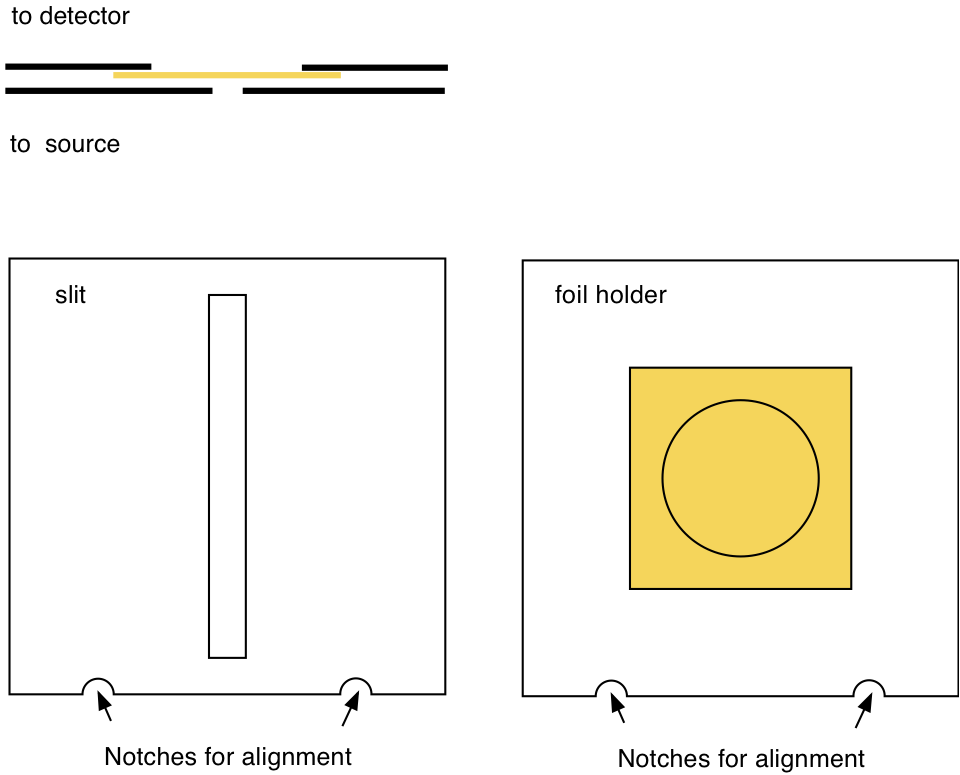
Fig. 20.3 Slit and target holder

20.3.2. Taking Data

1. Set the MCA live time to 300s and take a spectrum without target. You should see a peak, corresponding to the \(\alpha\) particles, which are mono energetic. The width of the peak is due to the thickness of the source itself where the \(\alpha\)-particles loose energy and the energy resolution of the detector.

2. Install the gold target with the 1mm slit (see Fig. 20.3). Make sure that the notches fit into their counter parts in the target holder. The large circle needs to face the detector and the slit faces the source.

3. Close the vacuum chamber, make sure the target position is at 0 degrees and pump down.

4. Take another spectrum. Note how the peak has shifted. This is due to the energy loss of the \(\alpha\)-particles in the target.

5. Take data at \(0^\circ, \pm 5^\circ, \pm 10^\circ, \pm 15^\circ, and \pm 20^\circ\). Select the acquisition times in such a way that you get about a 3% statistical error for \(0^\circ, \pm 5^\circ\). For \(\pm 10^\circ\) get 5% statistics and for \(\pm 15^\circ\), about 7% and about 10% or better for the rest. (Hint: remember a good estimate of the uncertainty of counts \(\sigma_N = \sqrt{N}\) where \(N\) is the number of counts observed)

6. For \(-30^\circ\) count for 20 minutes and if time allows for \(-40^\circ\) count for 0.5h. This assumes that at negative angles you measure higher count rates than for positive angles.

Remember: save all the spectra as SPE (ASCII) files. In that way you

can analyze them later using the LabTools package.

20.4. Analysis

Fig. 20.4 shows an example spectrum with the gold foil at 0 degrees.

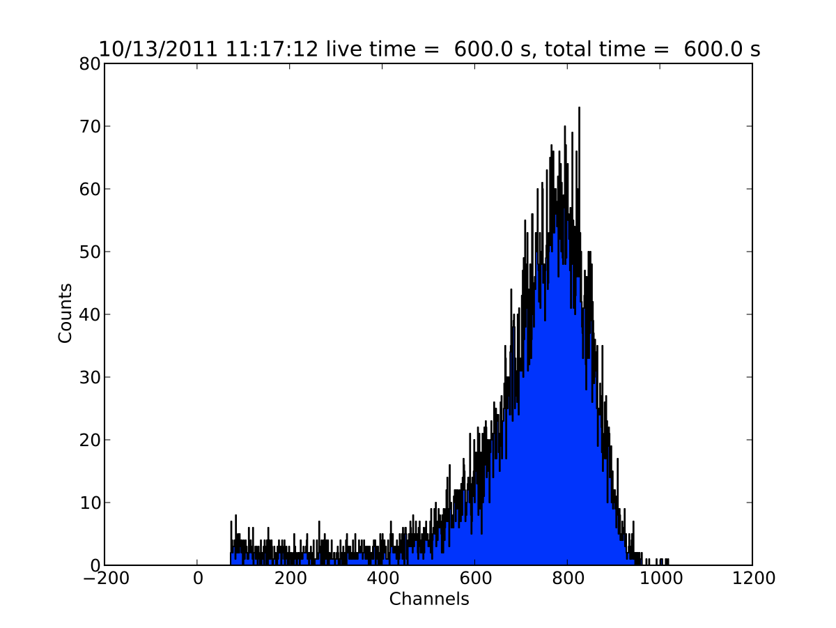
Fig. 20.4 Au spectrum at 0 degrees

1. Determine the count rates (counts/time) for each angle.

2. Check if you observe indeed Rutherford scattering by calculating the logarithm of the count rate (and its error) and plot this versus the logarithm of \(sin(\theta/2)\). You should see a linear relation ship. Make sure you take the absolute value of \(\theta\). You will most likely see that the rates left and right for the same angle are different. This is due to a possible offset in your angle measurement. Try to add or subtract \(\approx 2^0\) and see if the results improves. Determine above which minimum scattering angle \(\theta\) you probably see a linear relationship.For those angles fit a line and determine the slope. Does it agree with what you would expect for Rutherford scattering ?

3. To accurately determine the angle offset you will determine the coefficients in equation (20.3) , namely \(C\) and \(\theta_0\), via a non-linear fit of the experimental count rates. Then make a semi-log plot of the count rate as a function of \(\theta\) and plot the fitted curve. Discuss your observations and results.

20.4.1. Analysis Hints

20.4.1.1. How to sum bins in a histogram

For each spectrum add the counts in the peak. As this is a simple spectrum with only one peak, you can basically just add all channels (or bins) above a certain value. For the example in Fig. 20.4, you could add the channels between 400 and 1000. Assuming the spectrum is called sp when you load it, you get this sum with the command:

C, dC = sp.sum(400, 1000) # sum the channels between 400 and 1000
C, dC = sp.sum(200) # sum all channels above 200

Here C is the sum and dC is the uncertainty in the sum.

20.4.1.2. How to get the live time of a spectrum

The live time is stored in the title of the spectrum. The function below allows you to extract the number from the title:

# get the live time from a spectrum
def get_time(sp):
    tt = float(sp.title.split('=')[1].split('s')[0])
    return tt
#

Put this in your analysis script and you can get the time by doing:

t = get_time(sp)   # get the time
R = C/t            # calculate the rate
dR = dC/t          # calculate the error in the rate

20.4.1.3. How to do the non-linear fit

In order to determine the parameters of the angular distribution you need to define the function and its parameters. This is done as follows (please see General Non-Linear Fitting for more explanations):

C = B.Parameter(10., 'C')       # define the parameter
t0 = B.Parameter(0., 'theta_0') # define parameter for

def S(x):                       # define the function
    return C()/B.np.sin(0.5*(x - t0()) )**4

With these definitions you are ready to carry out the fit:

sfit = B.genfit( S, [C, t0], \
                 x = theta_r,\
                 y = R,\
                 y_err = dR)

Where the fit results are stored in sfit, theta_r is the scattering angle in radians, R the experimental rates and dR the uncertainties. Make sure that these arrays contain only those values that you want to use in the fit.

20.4.1.4. How to do a semi-log plot of data and fit

First plot the data as a semi-log plot:

B.plot_exp(theta_r, R, dR, logy=True)