19. PN-Junction

19.1. Background

The purpose of this experiment is to measure the voltage-current characteristics of a germanium diode and the way in which these characteristics vary with temperature. From these measurements, it will be possible to obtain a value for the energy gap in germanium and an order of magnitude estimate of Boltzmann’s constant.

At room temperature, an n-type semiconductor (e.g. germanium doped with arsenic) has electrons available for conduction whose energies lie in the conduction band. Conversely in a p-type semiconductor (e.g. germanium doped with gallium), conduction is by “holes” (vacancies due to missing electrons) in the valence band. When two such semi-conductors are joined to form a p-n junction, electrons will diffuse from the n to p side and holes from the p to n side provided they have enough energy to overcome the potential “hill”. The net diffusion current is

(19.1)\[I_{Dif} = I_{eDif} + I_{hDif} = C_1 e^{-eV_J/kT}\]

where \(V_J\) is the voltage across the junction and \(C_1\) is a constant, see Fig. 19.1. Because of this current, the p-side of the junction becomes negatively charged and the n-side positively charged. This results in a strong electric field pointing from the n- towards the p-side.

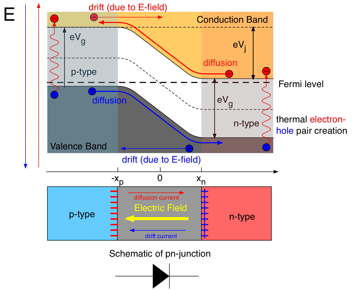
Fig. 19.1 Energy band diagram for a p-n junction.

Electron-hole pairs are also being thermally generated in both p and n regions with a probability of \(e^{-eV_g/kT}\), where \(eV_g\) is the energy gap between the valence and conduction bands. The electric field, mentioned above, will cause the holes in the n-side to flow towards the p-side and electrons from the p- to the n-side. This constitutes an “equilibrium drift current”:

(19.2)\[I_{Dr} = I_{eDr} + I_{hDr} = C_2 e^{-eV_g/kT}\]

At equilibrium, when no external field is applied the two current have the same magnitude \(I_{Dif} = I_{Dr} = I_0\), but flow in opposite directions. When an external field is applied the energy levels change as shown in Fig. 19.2:

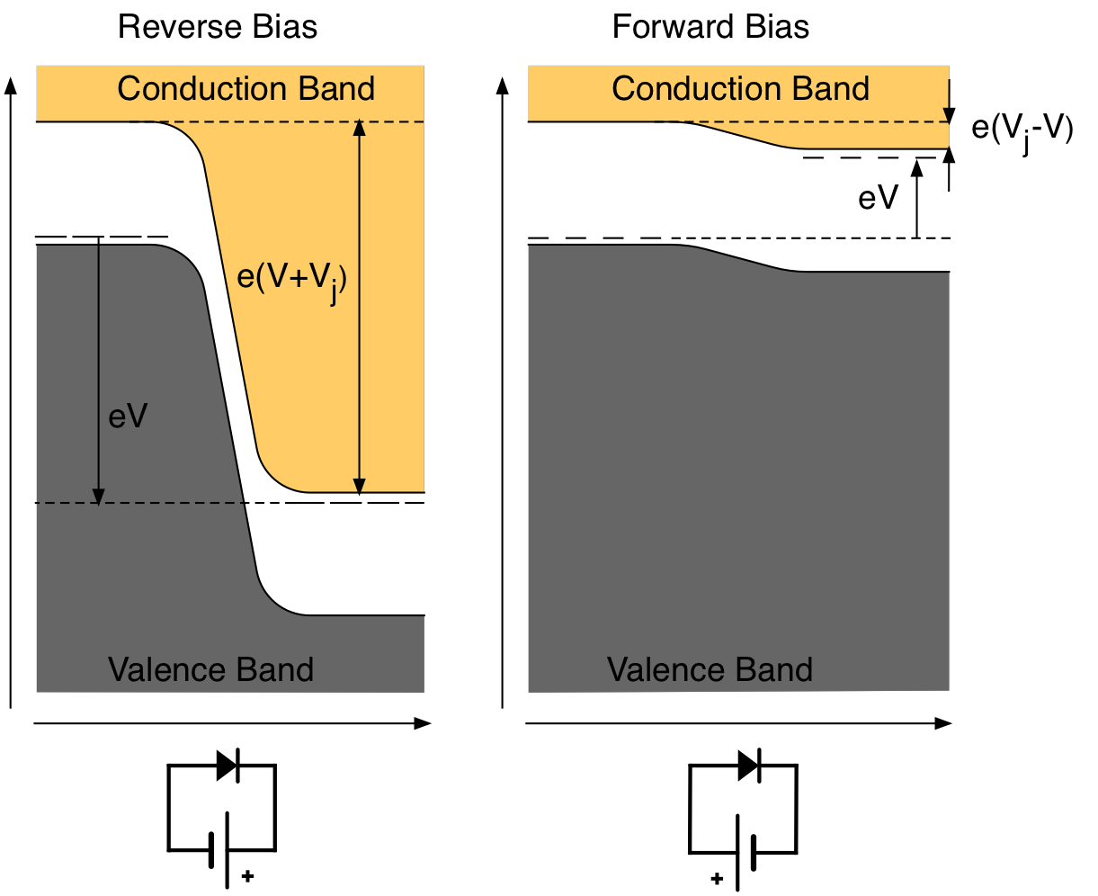
Fig. 19.2 Effect of reverse voltage (left) and forward voltage (right)

Therefore,

(19.3)\[ \begin{align}\begin{aligned}I_{Dif} = C_2 e^{-eV_g/kT} = C_1 e^{-eV_J/kT} = I_{Dr} = I_0\\e^{-(V_J - V_g)/kT} = const.\end{aligned}\end{align} \]

If an external voltage, V, is applied to the junction, with the p-side positive, the situation will be as shown in Fig. 19.2 The diffusion current will be increased by a factor, \(e^{e(V-V_J)}/e^{-eV_J/kT}\) leading to a a net forward current of

(19.4)\[I_f = I_{Dif} e^{eV/kT} - I_0 = I_0(e^{eV/kT} - 1)\]

Similarly if the external voltage is reversed, the net reverse current is

(19.5)\[I_r = I_0(1-e^{-eV/kT})\]

Both (19.4) and (19.5) may be written as a single equation

(19.6)\[I = I_0(e^{eV/kT} - 1)\]

where \(I\) represents the current from the p-side to the n-side and V is positive when it represents the forward voltage and negative for the reverse voltage.

19.2. Experimental Procedure

1. Forward and reverse characteristics at room temperature:

   Turn on the temperature control unit and set the temperature switch to \(25^oC\). The power supply for the p-n junction has two independent outputs and two independent voltage control knobs for forward and reverse operation respectively. Connect the leads from the junction to the FWD VOLT output jacks, matching red to red and black to black. Set the switch on the front panel to FWD. Turn both knobs fully anti-clockwise and switch on the unit. When the temperature has stabilized at \(25^oC\), take a series of current readings for voltages of 0.20, 0.22, 0.24, …. 0.30, 0.35, 0.40, 0.50, 0.60, …. 1.0 V. The digital display is in amps. Turn the knob back to zero and switch off the power supply. Now connect the junction leads to the REV VOLT output jacks red to black and black to red. Set the switch on the front panel to REV and switch on the unit. Record the current for voltages of 0.2, 0.4, …. 1.0, 2.0, 5.0, 10.0, 15.0, …. 40.0 V. The digital display is now in \(\mu A\).

2. Variation in reverse current with temperature:

   Set the reverse voltage at 10 V and record the current. Set the temperature switch to \(75^oC\) and record the current every \(5^oC\) as the junction warms up. You will probably find the current reading goes off scale at around \(65^oC\).

3. Forward characteristic at \(75^oC\):

   Switch off the power supply and reset the system for applying forward voltages. When the temperature has stabilized at \(75^oC\), determine the forward characteristic only as in part a.

19.3. Analysis

• To illustrate the rectifying properties of a junction diode, plot graphs of current (y-axis) vs voltage (x-axis) for both the forward and reverse conditions at \(25^oC\).

• From equation (19.6), \(ln (1 + I/I_0) = eV/kT\). Since \(I/I_0 >> 1\) over the range of forward measurements, \(ln(I) - ln(I_0) \approx eV/kT\). At a given temperature, \(I_0\) is a constant and so a graph of \(ln(I)\) vs \(V\) has a slope of \(e/kT\).

  Plot such a graph (including error bars) showing the forward characteristics at both \(25^oC\) and \(75^oC\) and use the slopes to determine Boltzmann’s constant. (Note that \(T\) is in kelvin.)

  In practice, the measured voltage includes the potential difference across the bulk of the semiconductor as well as contact potentials where the metal wires are joined to the semiconductor. The latter are small and the effects of the former can be minimized by taking the slope at small currents where the product \(IR\) will be small. You can still expect to get only an order of magnitude estimate for \(k\).

• Also from (19.6),it may be noted that for reverse voltages, \(V\), of –1 Volt or more, \(|I| \approx I_0\). This is the reverse saturation current measured in section b) which should have changed little with voltage.

  From (19.2), \(ln(I_0) = ln(I_{Dr}) = ln(C_2) – eV_g/kT\).

  Using the data in part b), plot \(ln(I_0)\) (y-axis) vs \(1/T\) (x-axis) [T in kelvin]. Using the accepted value of Boltzmann’s constant, obtain the energy bandgap, \(eV_g\), for germanium including its error.

  Include error bars in all your data points and the derived quantities.