18. The Photo-Electric Effect

18.1. Background

The experiment serves to demonstrate the photoelectric effect, for which Einstein was awarded a Nobel prize, and in the process determine Planck’s constant, \(h\).

The photoelectric effect is the process whereby a photon of energy \(E=h\nu\), incident on the surface of a conductor, transfers its energy to one of the electrons of an atom. If the energy is sufficient, the electron can not only escape from the material, but do so with a certain amount of kinetic energy. If the electron is in the highest available energy state within the conductor, the least amount of energy, \(\phi\), is needed to free it, and it will escape with the maximum kinetic energy. \(\phi\) is called the work function of the conducting material.

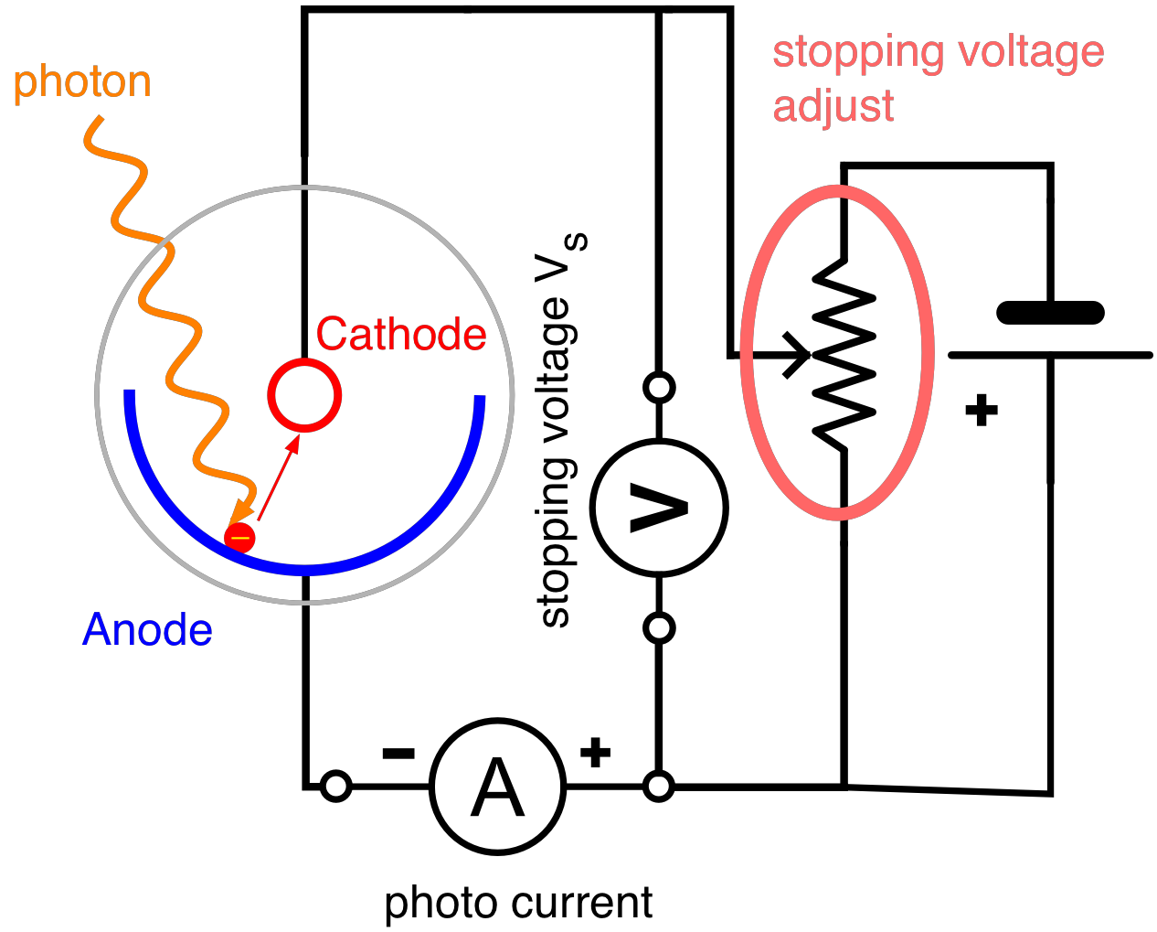
Fig. 18.1 Schematic of the photo-electric effect experiment. A photon hits the conducting anode and knocks out an electron. All electrons that have sufficient kinetic energy to reach the cathode produce an electric current. The adjustable stopping voltage determines the minimal kinetic energy the electrons need.

If the conductor forms the anode of a phototube, as shown in Fig. 18.1, no electrons will reach the cathode if the potential difference (retarding potential) between the anode and cathode is adjusted to the minimum value necessary to stop the fastest electrons. The loss of kinetic energy is then balanced by the gain of potential energy, \(e V_s\), and the energy equation is given by

(18.1)\[h\nu = e V_s + \phi\]

where \(V_s\) is called the stopping potential. The threshold frequency, \(\nu_0\), is the minimum photon frequency capable of eliciting the photoelectric effect. It is obtained by setting \(V_s = 0\) in equation (18.1):

(18.2)\[\nu_0 = \frac{\phi}{h}\]

In the experiment, a monochromator is used to isolate a number of different wavelengths from a mercury lamp, and for each the stopping potential is determined. From the data, \(h\), \(\phi\), and \(\nu_0\) may be determined.

18.2. Experimental Equipment

The setup for this experiment is shown in Fig. 18.2. It consists of a mercury lamp, a monochromator, the photocell with a control for the stopping voltage and a current amplifier with a zero adjust for the photo-current measurement. Be careful with the mercury lamp. It is made of quartz, emits UV and gets very hot.

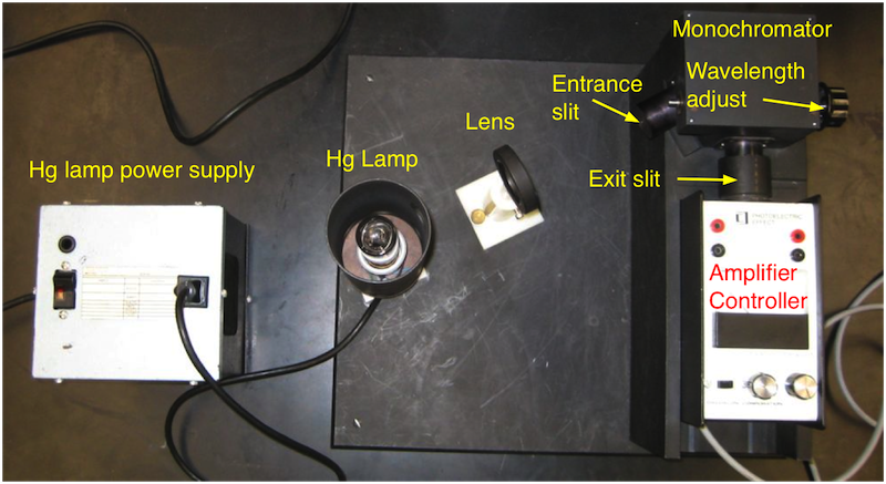
Fig. 18.2 Overview of the main equipment parts of the photo-electric effect experiments.

You will also need two additional digital multimeters to measure the stopping voltage and the photo current. A close-up of the instrument is shown in Fig. 18.3.

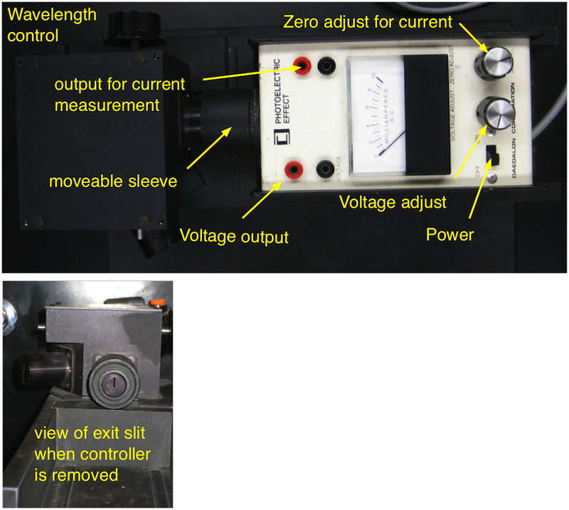
Fig. 18.3 The monochromator and the instrument containing the photocell. The instrument can be removed when the sleeve is pushed toward the monochromator. Then the exit slit can be viewed to select which Hg spectral line is used. Then you remove the instrument make sure that it is either turned off or that the stopping voltage is at a maximum (know turned CW as far as it goes)

The wavelength can be adjusted by turning the knob at the side if the monochromator (this rotates the grating inside the monochromator). An arrow indicates the direction towards shorter \(\lambda\).

18.3. Pre-Lab Preparation

1. Assume you have determined that the stopping voltage for the yellow light is 0.5V and it is 1.5V for the ultraviolet light. Determine the value of hc? The wavelengths of the mercury spectrum can be found in the manual. Express the results using the unit of ev*nm.

2. Prepare the data file formats for each wavelength and store the wavelength as a parameter in the header section.

3. Prepare a python script to plot your data while you are taking them. This makes sure that you have good quality data.

18.4. Experimental Procedure

DAMAGE COULD RESULT IF THE UNIT IS TURNED ON WHILE THE PHOTOELECTRIC CELL IS EXPOSED TO ROOM LIGHT OR INTENSE LIGHT

1. Turn on the mercury lamp and wait for about 5 minutes until it reaches its full intensity. Connect one of the digital multimeters to measure the retarding potential and set it to the 20 V DC range.

2. Connect the second multimeter to measure the photoelectric cell current (thereby duplicating the reading on the less accurate built-in milliammeter) and set it to the 2 mA DC range.

3. By turning the wavelength control on the side of the monochromator, different spectral lines will become visible at the exit slit. Those to be used are: yellow (578 nm), green (546 nm), blue (436 nm) violet (405) and ultra-violet (365 nm). The violet appears relatively faint and the ultra-violet is, of course, invisible.

4. Adjust the wavelength control until the yellow line is visible.

5. Place the photoelectric cell on the stand forming a light tight seal with the monochromator.

6. Turn the “voltage adjust” control fully clockwise (maximum retarding potential) and then switch on the power switch.

7. Cover the entrance slit of the monochromator to prevent light entering and adjust the “zero adjust” until zero current is obtained. This is a very delicate adjustment and you may not be able to obtain a precise zero.

8. Let the light back into the system. Turn the “voltage adjust” control in a counter-clockwise direction, thereby reducing the retarding potential, until a current of about 1 mA is registered. Now adjust the wavelength control until the current is maximum. You have now optimized the monochromator for 578 nm.

9. Turn the “voltage adjust” control fully clockwise (maximum retarding potential) Before recording the “stopping potential”, double check the zero setting, blocking the light as before. After you let the light back into the system you will notice a small negative current which is normal. Try to figure out where this current is coming from.

10. Measure the current as a function of the retarding potential by reducing the retarding voltage first in step of 0.5 V and as soon as you see a noticeable change in the photo current decrease the voltage steps in such a way that you have about 10 measurements in the ‘knee region’ and data up to a current of about 0.5 mA. You should end up with about 15 - 20 data points for each color.

11. Having completed this wavelength, turn the “voltage adjust” control fully clockwise and remove the photoelectric cell so that you can adjust the monochromator for the next spectral line. Repeat the above procedures for each line in turn. The ultra- violet line will have to be found by adjusting the wavelength control beyond the position for the violet line until a current is registered. Keep adjusting the “voltage adjust” control to prevent the current reading from going off-scale while seeking the maximum current.

18.5. Analysis

The goal of the analysis is to carefully determine the minimal retarding voltage from which one can determine kinetic energy of the ejected photo-electrons.

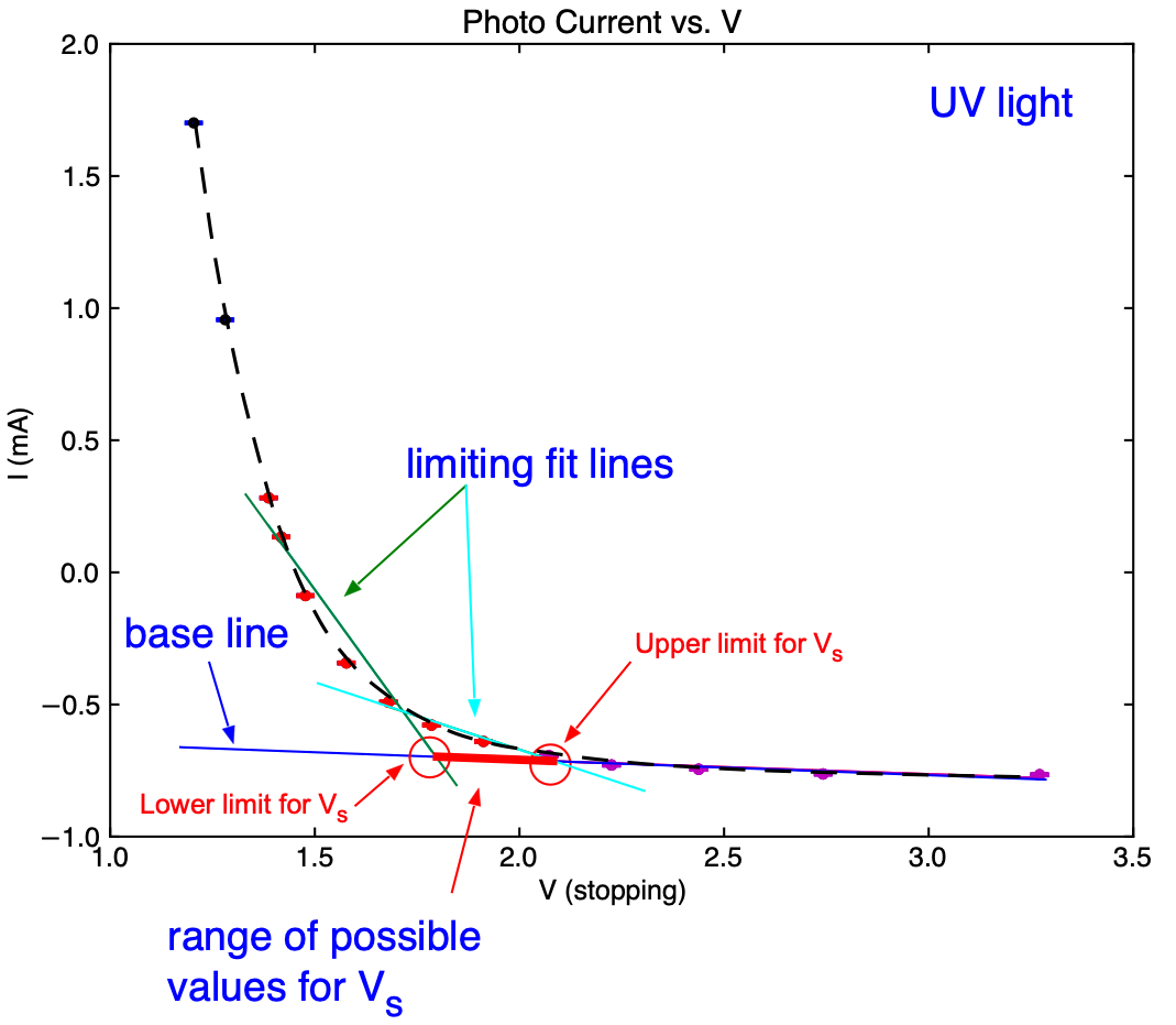
Fig. 18.4 Typical current vs. stopping voltage (\(V_s\)) curve for the UV line. Note the ‘knee` and the two limiting lines fitted to determine the range of values for the stopping voltage.

Each data set taken for a specific wavelength needs to be analyzed separately and the general method is as follows:

1. Plot the measured current, \(I\) as a function of the stopping potential \(V_s\). A typical example is shown in Fig. 18.4. Note that the current increases smoothly and it is not obvious how to determine the exact value of the minimal value of \(V_s\). A possibility is so fit a line to the data where \(V_s\) is large and the current changes only lightly. In the area where you see the ‘knee’ in the curve select a second range of points where the current starts to rise (typically a current increase of 200 - 400 \(\mu A\) works well). Fit a second line to these data and calculate the intersection of the two lines. The value for \(V_s\) at the intersection can then be interpreted as the minimal stopping potential to prevent electrons from reaching the anode and the potential energy of the electrons when they just reach the anode corresponds to their kinetic energy when the were just ejected from the cathode. In order to get an estimate of the uncertainty use limiting cases in your selection of data points to determine these two lines (see Fig. 18.4 )

2. Use the voltages and their uncertainties determined in the previous step to determine \(h\) and \(\phi\) by fitting a line to the measured electron energies as a function of the frequency of the light.

3. Why to you measure a current in the opposite direction of the photo current when \(V_s\) is maximal and you carefully zeroed the current measurement.

18.5.1. Analysis hints:

How to fit a line to a subset of data of \(I\) and \(V\) ?:

Select the data using:

In [1]: ir = B.in_between(-0.1, 0.3, I)         # select current between -0.1 and 0.3
In [2]: l1 = B.linefit(V[ir], I[ir], sig_I[Ir]) # fit the line

Here ir contains the information on the data where the current I is between -0.1 and 0.3. The fit results are stored in l1. The most important are: l1.slope and l1.offset and their uncertainties, l1.sigma_offset and lq.sigma_slope. For further information check the general documentation.

If you prefer to select data using the voltage you would do:

In [1]: vh = B.in_between(1.5, 3.5, V)           # select voltages between 1.5 and 3.5
In [2]: l2 = B.linefit(V[vh], I[vh], sig_I[vh]) # fit the line

Here vh contains the information on the data where the voltage V is between 1.5 and 3.5 and the fit results are stored in l2.

Instead of using B.in_between you can also do:

In [1]: vh = (1.5 <= V) & ( V<= 3.5)            # select voltages between 1.5 and 3.5
In [2]: l2 = B.linefit(V[vh], I[vh], sig_I[vh]) # fit the line

which is what B.in_between actually does.