17. Lenses and Optical Instruments
17.1. Background
Lenses and mirrors are key parts in optical instruments that played and continue to play a pivotal role in research and the development of our current scientific understanding of the world. This Lab consists of a series of small experiments that give you the opportunity to use and test the thin lense equation, measure the focal length of lenses, assemble and measure the magnification of a microscope, a telescope and a slide projector. To understand how these instruments work and to model their properties we use geometric optics and ray tracing. Geometrical optics was covered in your introductory physics class (PHY 2049). If you did not cover this material, please read up on it in your book or in this OpenStax Online Book
17.2. Raytracing and the Lens Equation
In the following all lenses are assumed to be infinitely thin meaning that the finite thickness of the glass has been ignored. This is most of the time a good approximation for single lenses and when the radii of curvature of the two lens surfaces and are much larger than the actual thickness of the lens. We are also restricting the analysis the rays that are close to the optical axis and make only small angles \(\theta\) with respect to the optical axis such that \(\tan{\theta} \approx \sin{\theta} \approx \theta\).
To study the optical propertyies we use so-call light rays. Light rays are lines perpendicular to wave fronts (surfaces of constant phase) and indicate the direction of energy flows. For instance plane waves correspond to parallel rays while spherical waves have rays originate or converge to a point. Following the path of a light ray and applying the laws of reflection and refraction allows one to study the optical properties of even complex optical systems.
The effect of a thin lens on a light ray cab be characterized by the following two rules (Fig. 17.1 and Fig. 17.2):
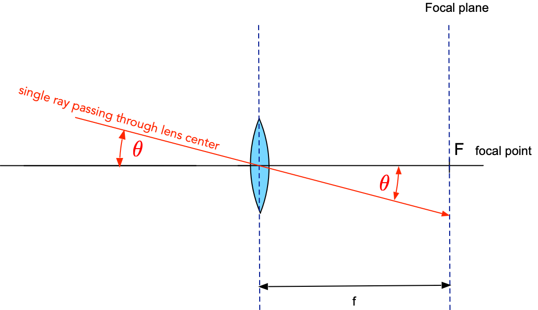
Fig. 17.1 Rule 1: A ray that passes through the lens center, i.e. where the lens intersects the optical axis, is not deflected.
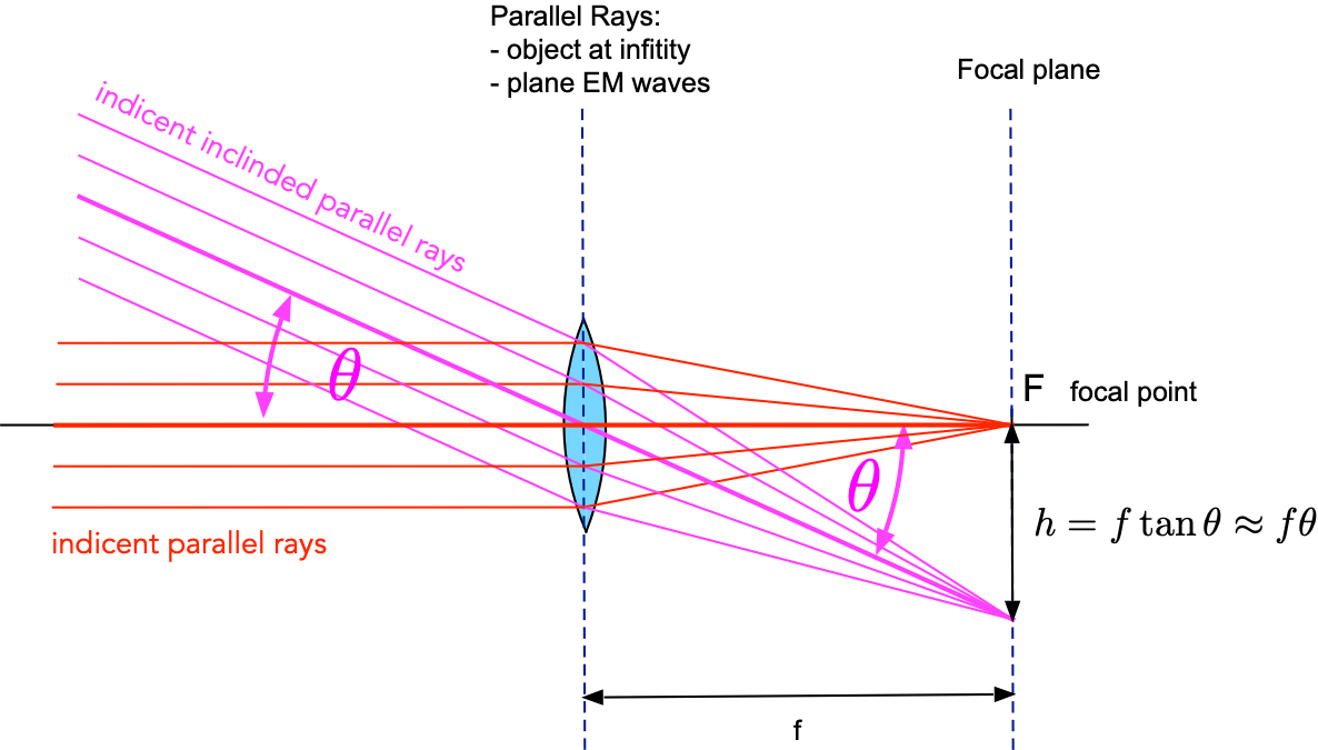
Fig. 17.2 Rule 2: Parallel rays intersect at a point in the focal plane.
These two rules allow one to study image formation by a single lens. The basic elements for analyzing image formation by a single lens are shown in Fig. 17.3. The lens surfaces are spherical segments and defined by their radius of curvature. The line defined by the two centers of curvature \(R_1\) and \(R_2\) is the optical axis.
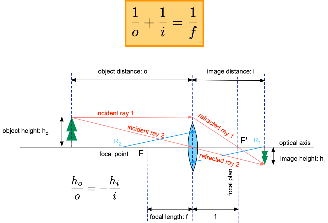
Fig. 17.3 Image formation by a single lens. \(F, F'\) indicate the focal points and \(R_1, R_2\) are the center of curvatures for each lens surface.
To find the location of an image of an object of heigh \(h_o\) located a distance \(o\) from the lens (i.e. the fir tree in Fig. 17.3) one follows two incident rays originating from a point of the tree. Ray 1 is parallel to the optical axis and ray 2 passes through the center of the lens. After the lens ray 1 passes through the focal point \(F'\) while ray 2 passes undeflected through the center of the lens (this is because the lens is infinitely thin). The two rays intersect at the location of the image a distance \(i\), the image distance, behind the lens. The relation between object distance, image distance and focal length is given by the lens equation (17.1):
From ray 2 in Fig. 17.1 one can understand the definition of magnification \(m\):
Where the negative sign indicates an inverted image. Based on these two equations the basic principle of the magnifier, the microscope, the telescope and many other instruments can be understood. Since every leans is characterized by its focal length it is important to be able to measure this quantity. One can find the pth of any ray through a lens by drawing an imaginary, parallel ray to the indicent ray that passes through the lens center. The imaginary ray and the original ray join in the focal plane of the lens thud determining the direction of the indicent ray after the lens.
17.3. Lens Combinations: The Lens Doublet
By combining lenses their range of applications is dramatically increased. A modern zoom lens is typically a combination of 10 lenses grouped in pairs and triplets. The most basic combination is the lens doublet consisting of two lenses with focal lengths \(f_1\) and math:f_2 separated by a distance \(d\). Using the same trechnique as described above we can find the intersection of three parallel rays and thus the focal plane of this combination as is shown in Fig. 17.4.
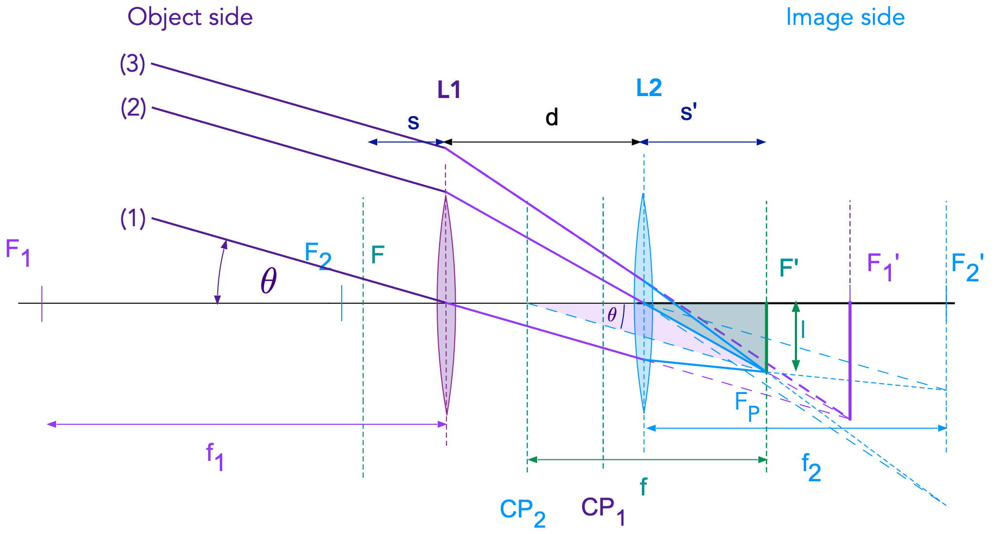
Fig. 17.4 Three parallel rays enter a lens doublet from the left. Ray (1) passes through the center of L1, ray (2) passes throuh the center of L2 and ray (3) is a general ray. All rays converge at the focal point \(F_P\) in the focal plane located at \(F'\). The focal length of the doublet \(f\) is the distance between the focal plane and the so-called second cardinal plane (\(CP_2\)).
Tracing the rays, following the rule for thin lenses, one sees that they all intersect at point \(F_P\) which defined the focal plane (the plane perpendicular to the optical axis). All parallel rays entering the doublet will be focused to a point in this plane. The focal length \(f\) in general is defined as follows for parallel rays originating from an infinitely distant object:
where \(I\) is the distance of the focal point \(F_P\) from the optical axis, or in other words the image size of an object that is inifinitely far away. Drawing a line through \(F_P\) and parallel the incident rays, it intersects the optical axis at the so-called second cardinal point \(CP_2\). The plane perpendicular to the optical axis through this point and is called the second cardinal plane. The distance between the focal plane and the second cardinal plane is the focal length \(f\) of the doublet. Thie distance \(s'\) is the distance between the lens \(L_2\) and the focal plane, also called the back focus distance.
In Fig. 17.5 a similar construction is shown for rays entering the doublet from the image side and converging in the focal point \(F\) on the object side. Here \(s\) is the distance of \(F\) from the front lens \(L_1\). Note that \(s\) is different from \(s'\) in Fig. 17.4. The first cardinal point \(CP_1\) is a distance \(f\) away from the focal point toward the image side.
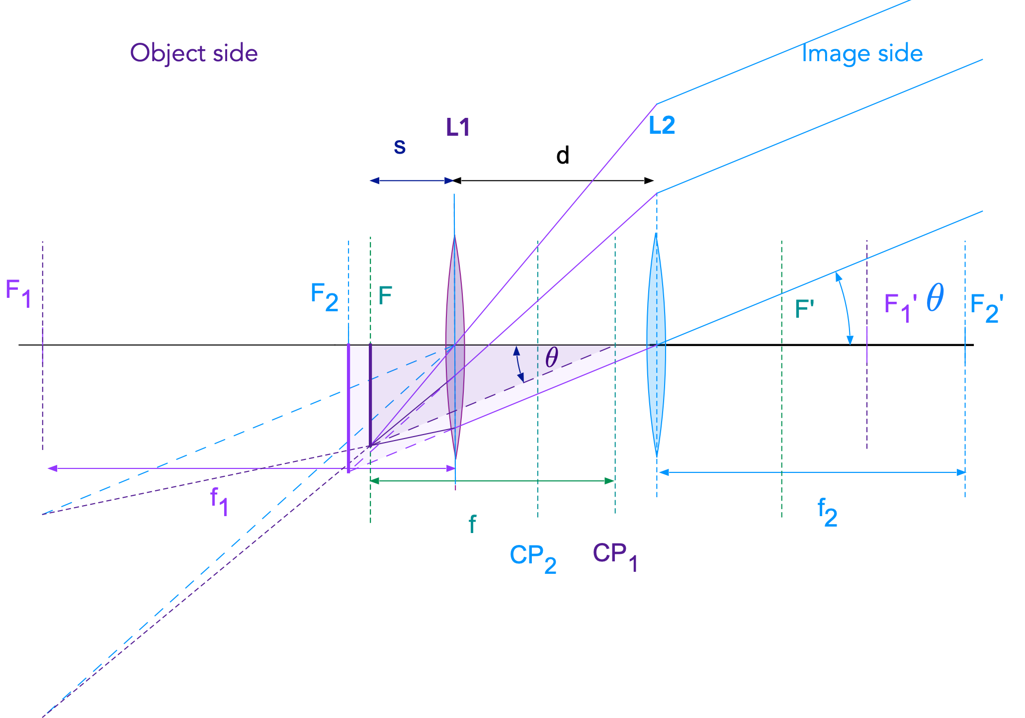
Fig. 17.5 Similar to Fig. 17.4, but for rays entering from the image side. This defined is object side focal point and the first cardinal point and plane.
If the refractive index on the object side and the image side are identical then the cardinal points are identical to the so-called nodal points. The nodal points have the following property: If a ray enters the first lens \(L_1\) in such a way that its extension would intersect the first nodal point \(NP_1\) the ray is exiting the dublet at lens \(L_2\) as a parallel ray to the incident on and originating from the secont nodal point \(NP_2\). As mentioned prefore these points are identical to the cardinal points \(CP_1\), \(CP_2\) in all out experiments. This is illustrated in Fig. 17.6.
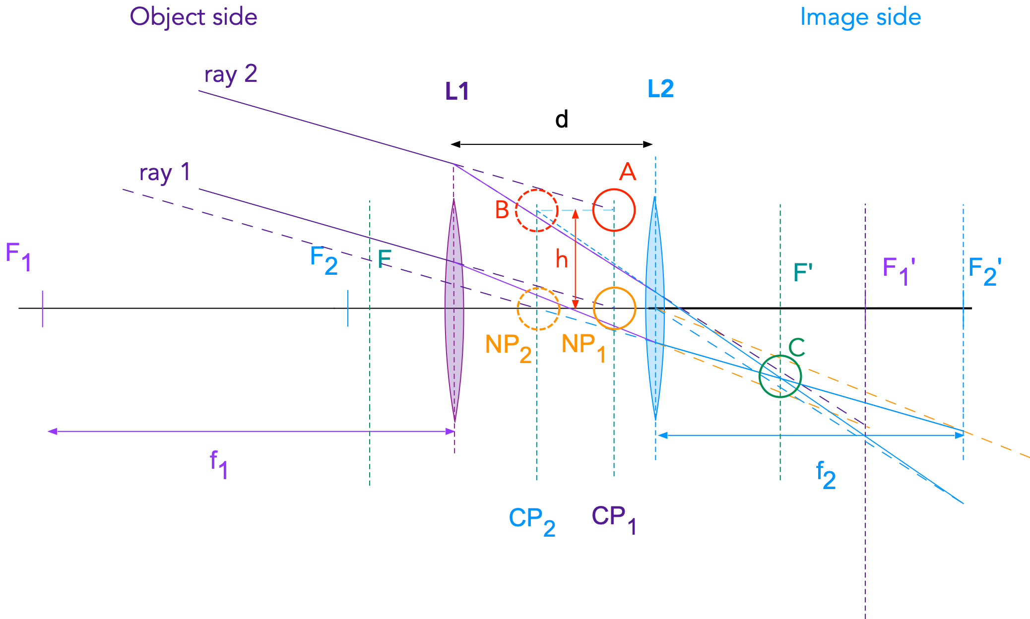
Fig. 17.6 Ray 1 enters \(L_1\) and its extension would intersect the optical axis at the first nodal point \(NP_1\) = \(CP_1\) (orange circle). The exiting ray 1 is parallel to the original one and intersects the optical axis at the second nodal point \(NP_2\) = \(CP_2\) (dashed orange circle).
Cardinal points/planes and nodal points/planes play a crucial role in image formation for doublets. For example Ray 2 in Fig. 17.6 is parallel to ray 1 and would intersect the first cardinal plane a point \(A\) a distance \(h\) from the optical axis (red circle). After exiting the doublet ray 2 is defined by 2 points. The first point is on the second cardinal plane (\(CP_2\)) a distance \(h\) from the axis (point \(B\), red dashed circle) and the second point is the intersection of ray 1 with the focal plane (point \(C\), green circle). Therefore there are two rules for doublets:
A incident ray that would hit the first nodal point leaves the doublet as a parallel ray originating from the second nodal point.
A general indicent ray that intersects the first cardinal plane at a distance \(h\) from the optical axis exits the double as a ray originating from the second cardinal plane at the same distance \(h\).
These two rules in combination with the known focal length of the dublet allowd one to construct the image formed by a doublet as shown in Fig. 17.7
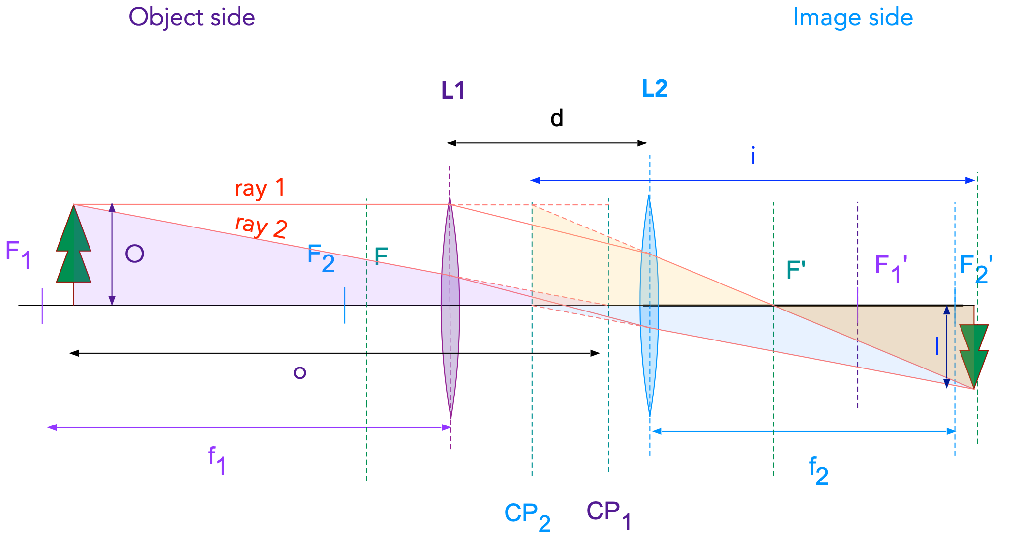
Fig. 17.7 Raytracing of two rays to constuct the image formed by a lens doublet. Ray 1 is parallel to the optical axis and intersects the optical axis at the focal point \(F'\) and ray 2 is incident on the first nodal point (\(CP_1\)) and leaves the doublet as a parallel ray originating from \(CP_2\). Where ther two rays intersect the image is formed.
From the similarities of the two pairs of triangles in Fig. 17.7 one can show that the lens equation for doublets is identical to the one for thin lenses, provided ones uses the definitions of objec and image distances as shown.
To summarize the optical properties of a lens double in regards to ray tracing and geometrical optics are determined by its focal length and the locations of the cardinal (and nodal) points. The locations of the caridnal points/planes can be constructed geometrically as shown in Fig. 17.8
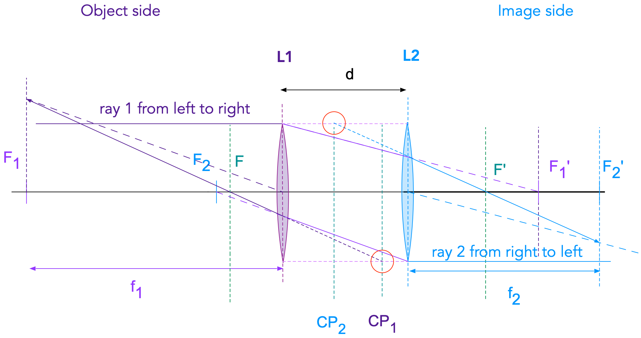
Fig. 17.8 Ray tracing to find the location of the cardinal planes of a lens doublet.
17.4. Focal Length Determinatio Part A
The simplest method to determine the focal length is to place an object and a lens at a known position and find the location of the object image on a screen. From the lens equation you would then find the focal length. The problem with this method is that it is difficult to determine the exact location of the lens and thus the object and image distances. A better method would be one where we do not need to measure the exact position of the lens but where one makes two measurements while the distance bweteen the object and the screen is kept fixed abd the lens has been moved. This is possible and the corresponding raytracing diagram is shown in Fig. 17.4.
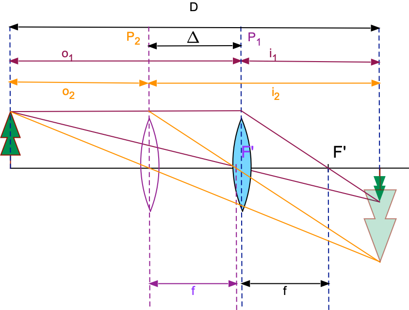
Fig. 17.9 Image formation for two lens positions when the object and image are a fixed distance \(D\) apart and the lens is moved a distance \(\Delta\).
Fits the lens is at position \(P_1\) with an object distance \(o_1\) making an image a distance \(i_1\) away from the screen. THe lens is then moved a distance \(\Delta\) toward the object until again an image appears on the screen. The lens is then at position \(P_2\) with an object distance \(o_2\) and an image distance \(i_2\).
From the following relationships:
and the lens equation show that (which means derive and show the steps)
17.5. Focal Length Determinatio Part B
THe above method does not work well for short focal lenths as one finds in eye pieces for microscopes or telescopes. Another possibility is bases on measuring the magnification of the lens.