13. Hydrogen Spectrum

13.1. Background

The Hydrogen atom is the simplest atom and plays a fundamental role in nature. It is basically the only neutral atomic two-body system and is therefore the only system that can be calculated exactly. All other (neutral) atoms contain more electrons and are therefore many-body systems requiring approximation methods of various degrees of sophistication in order to calculate their properties. Light emitted by a gas can be decomposed into its different wavelengths with a spectroscope. Early spectroscopes used a glass prism where the index of refraction depends on the wavelength (called dispersion) leading to different bend angles for different wavelengths. These studies were pioneered by Robert Bunsen and Gustav Kirchhoff in the middle of the 19th century. They observed that gases only emit at certain specific wavelengths called the spectral lines and that these lines are specific to each element. This made it possible to analyze the composition of substances using spectroscopes. Hydrogen, was found to have four visible lines and Johann Balmer was able to find a relationship to reproduce the observed wavelengths and to predict new lines outside of the visible spectrum. It later turned out that Balmer’s formula was a special case of Rydberg’s formula:

Johann Balmer’s Formula:

(13.1)\[\lambda = \frac{h m^2}{m^2 - n^2}\]

where \(n = 2, h = 3.6456\times 10^{-7} m\) and \(m = 3, 4, 5 ...\)

Note that \(h\) is Balmers constant and defined for \(n = 2\). As an exercise express \(h\) in terms of \(R_H\) and \(n_1\).

Rydberg’s Formula:

(13.2)\[\frac{1}{\lambda} = R_H \left( \frac{1}{n_1^2} - \frac{1}{n_2^2} \right)\]

where \(R_H\) is the Rydberg constant for Hydrogen.

These expressions can only be explained using a quantum mechanical model of the Hydrogen atom. Niels Bohr created the first quantum model for the binding energy of the electron in Hydrogen:

(13.3)\[ \begin{align}\begin{aligned}E_n = -\frac{k e^2}{2 a_B}\frac{1}{n^2},\\a_B = \frac{\hbar^2}{k e^2 m_e} = 5.29\times 10^{-2} nm\\R_H = \frac{k e^2}{2 a_B (h c)} = 1.1\times 10^{-2} nm^{-1}\end{aligned}\end{align} \]

where \(k\) is the constant used in calculating the potential energy of the electron (depending on the unit system used). For SI units: \(k = 1/4\pi \epsilon_0\) and \(a_B\) is the Bohr radius.

The observed light is produced by the emission of photons when an electron changes from an energy state \(E_1\) to another state \(E_2\) such that:

(13.4)\[ h\nu = \frac{h c}{\lambda} = E_2 - E_1\]

where \(h\) is Planck’s constant.

The goal of this experiment is to determine the wavelengths of the visible Hydrogen lines as accurately as possible, to determine which values \(n_1, n_2\) reproduce the data best and to determine the Rydberg constant (and therefore the ionization energy of the Hydrogen atom).

13.2. Experimental Equipment

For these measurements you will be using a Hydrogen lamp where a Hydrogen/Deuterium gas mixture is excited by an electric discharge. You will analyze the emitted light using a diffraction grating spectroscope and observe the spectral lines in the first and second diffraction order.

13.2.1. Spectroscope

The principle layout of the spectroscope is shown in Fig. 13.1

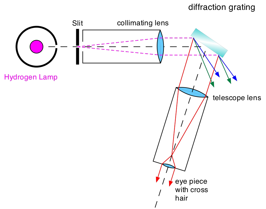
Fig. 13.1 Picture of the diffraction grating spectroscope.

Light from the Hydrogen lamp hits the entrance slit. The collimator lens produces a beam of parallel light incident on the reflection grating. The telescope lens produces an image of the entrance slit which is magnified by the eyepiece containing a cross hair. The angle under which the telescope observes the diffracted light with respect to the grating surface together with the incident light direction is used to determine the wavelength of the light as described below.

13.2.2. Principle of a Diffraction Grating

The diffraction grating consists of a reflecting surface containing many parallel grooves (the current grating has 1200 grooves per mm) separated by a fixed distance (the grating constant \(D\)). When an incoming plane wave (indicated by the parallel rays (1), (2) etc) hits the surface of the grating each groove acts as the source of an outgoing elementary wave. The entire grating then acts as an array of synchronous sources and the observed interference pattern can be understood as follows:

If we observe the scattered light at an angle \(\theta\) with respect to the normal of the grating surface, each outgoing ray (part of the original plane wave) has a path-length difference of \(\Delta = D \sin (\theta)\) with respect to its neighbor. The amplitude of the observed outgoing wave is the sum of the amplitudes of all the outgoing elementary waves taking into account their respective phase shifts. This can be calculated using phasors representing the amplitudes.

The intensity of the outgoing wave depends on the relative phase shift between the waves. For constructive interference one needs

(13.5)\[ \Delta = D \sin (\theta) = m_d\lambda\]

where \(m_d\) is an integer and \(\lambda\) is the wave length. How to calculate the intensity pattern of a grating with a total of \(N\) grooves is outlined in Fig. 13.2

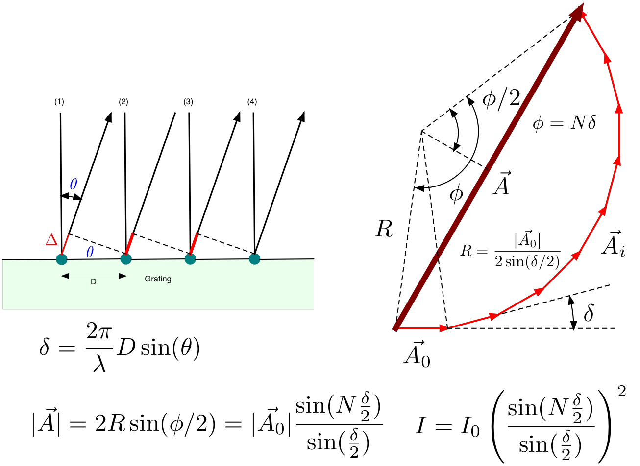
Fig. 13.2 Interference of several synchronous sources each with an amplitude \(|\vec{A_0}|\). The path length difference between adjacent rays is \(\Delta = D \sin (\theta)\) and the final intensity \(I = |\vec{A}|^2\).

As an example, Fig. 13.3 shows the distribution for \(N = 2\) and \(N = 16\). The grating used in this experiment has \(N = 30480\) with \(D = 1/1200\) mm. Since the sharp maxima for each wavelength occur when (13.5) is fulfilled, each wavelength has its peak at a different angle. The spectroscope measures this angle.

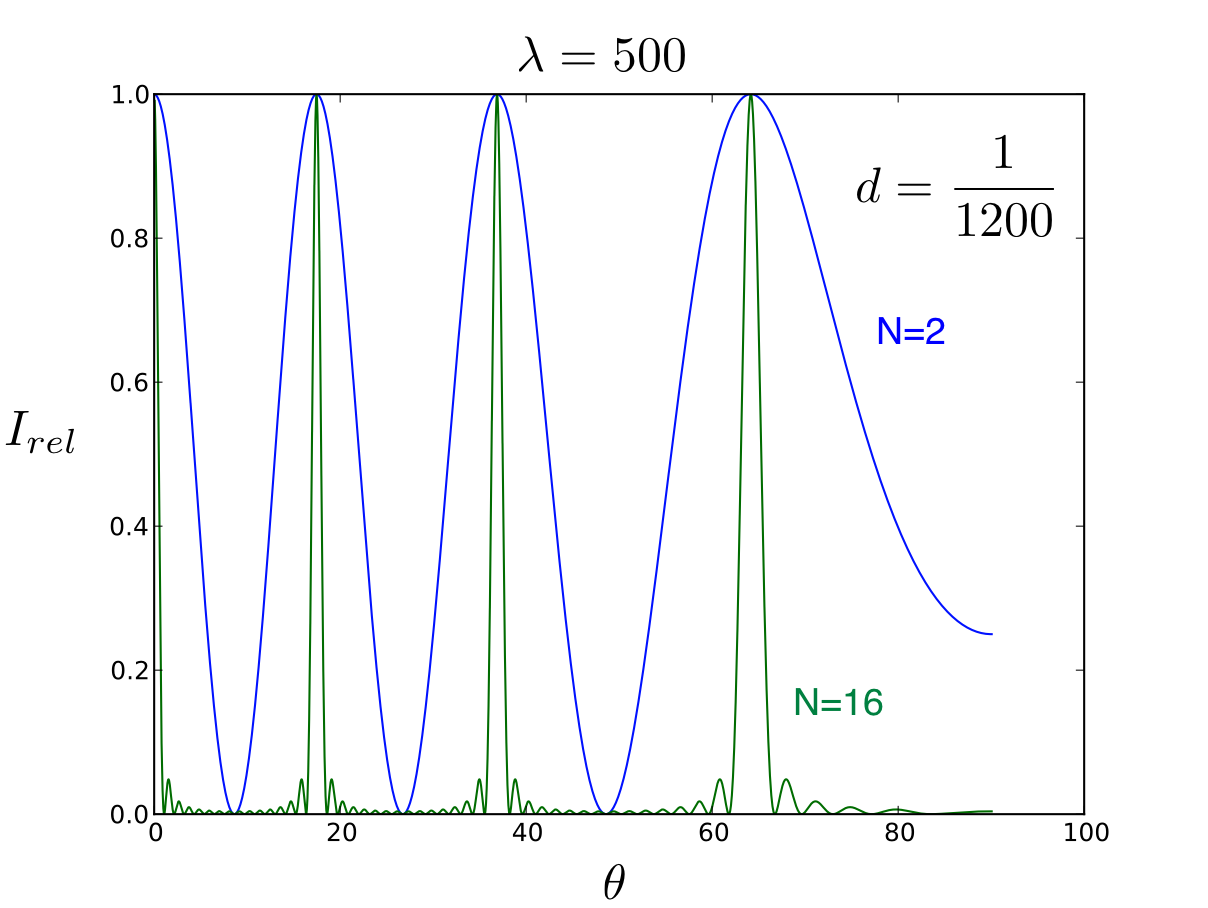
Fig. 13.3 Intensity distribution for a grating with \(N = 2\) and \(N = 16\). The grating constant is \(D = 1/1200\) mm. The \(\lambda\) is in nm and \(\theta\) in degrees.

13.3. Pre-Lab Preparation

1. Assume you observed the lamp image (without the grating) at \(180^\circ 4’\) Then you install the grating and saw the reflected lamp image (with the grating), or so-called \(0^{th}\) image, at \(163^\circ 45’\). After that, you observed a greenish blue light for the first time at \(106^\circ 2’\) . What is the wavelength of this greenish blue light? Results should in the unit of nm. And the grating spacing is 1/1200 mm.

13.4. Experimental Procedure

1. Turn on the hydrogen lamp and carefully remove the grating if it is still installed. DO NOT TOUCH THE GRATING SURFACE.

2. Place the lamp close to the slit and put the telescope on the opposite side as shown in part (a) of Fig. 13.4. Make sure you see a sharp image of the slit in the center of your eyepiece. Adjust the focus as necessary and make sure the cross hairs are sharp and vertical. Write down the angle of this configuration as you can read it from the angle scale with the help of the vernier (ask for help if necessary). Now you have determined the angle of the optical axis of your instrument. Fix it and DO NOT CHANGE IT ANYMORE.

3. Move the telescope by about 40 degrees (the exact number does not matter at this point; see (b) of Fig. 13.4). Insert the grating such that it;s surface is centered as much as possible on the center of the table. Carefully rotate the grating until you see again the image of the illuminated slit. Center the slit as well as you can. Write down the angle reading at this point as accurately as possible. DO NOT TOUCH the grating after this as it is aligned. You have now determined the angle \(\theta_0\). This angle is very important as it determined the incident angle of the light with respect to the grating surface. Now you are ready to observe the spectral lines.

4. Darken the room and carefully move the telescope until you see the first spectral line (typically the violet one). For each line write down the angle without changing the orientation of the grating or the original scale. The dark violet line is difficult to observe. You need to carefully cover the grating with the black cloth and adapt your eye to the dark. The blue-green and the red line are much easier to see.

5. Once you have recorded the angles for all 4 lines further increase the angle \(\theta\) until you see the violet line again. This is the second order. Try to measure as many lines as possible in second order.

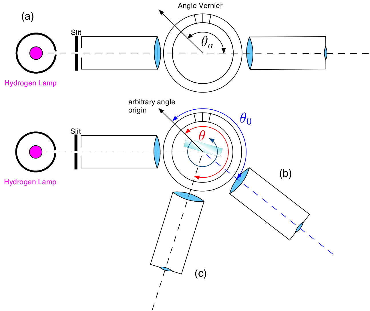
Fig. 13.4 Aligning the spectroscope. (a) Determine the angle of the optical axis. (b) Observe the 0th order and determine the angle \(\theta_0\). (c) Measuring spectral lines.

13.5. Analysis

In order to extract the wavelength from the angle measurements the geometry used in the spectroscope needs to be studied in detail. While the principle is the same as shown in Fig. 13.2 there is the important difference that the light is not incident perpendicular to the grating surface but and an angle \(\theta_{in}\) as shown in Fig. 13.5

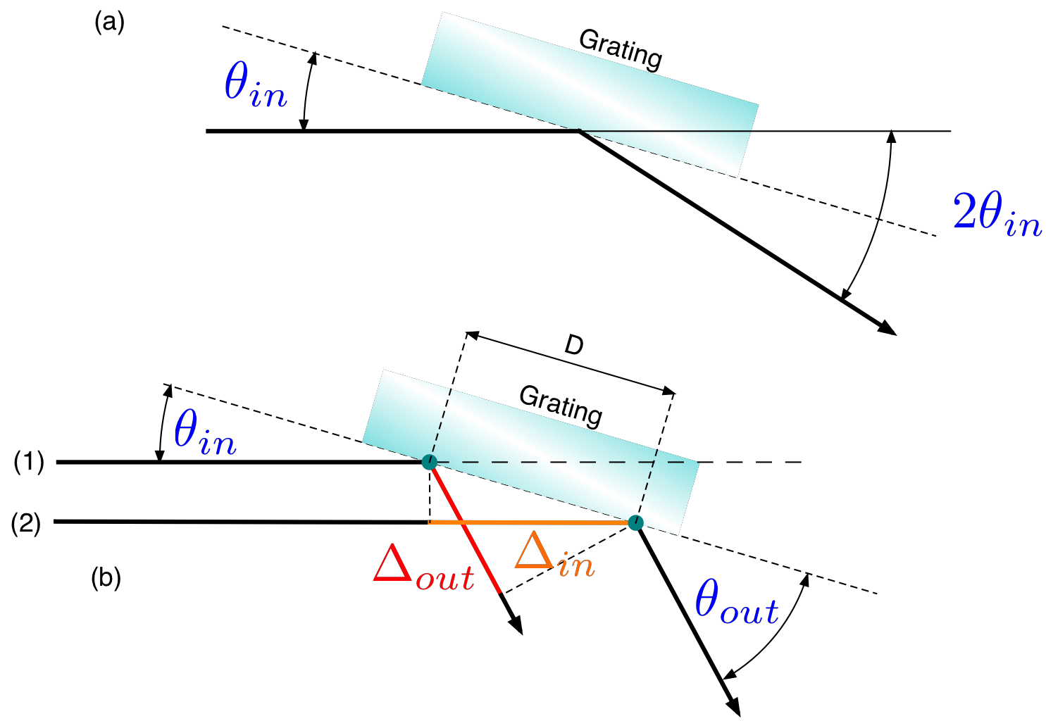
Fig. 13.5 The geometry of the incident and diffracted light. (a) The angle \(\theta_{in}\) can be determined from the angle measurements during the alignment procedure. (b) \(\Delta_{in}\) is the path length difference between the two incoming rays (1) and (2) and \(\Delta_{out}\) is the path length difference between the corresponding outgoing rays. \(D\) is the grating constant (distance between neighboring sources).

From the alignment measurement you know the angle \(\theta_a\) and \(\theta_0\). From these two you can get:

(13.6)\[ \begin{align}\begin{aligned} \theta_{in} = \frac{\theta_0 - \theta_a}{2}\\ \theta_{out} = \theta - (\theta_a + \theta_{in})\\ \theta_{out} = \theta - \frac{\theta_0 + \theta_a}{2}\end{aligned}\end{align} \]

As the incident light makes an angle \(\theta_{in}\) with respect to the grating surface there are now 2 path length differences to take into account:

(13.7)\[ \begin{align}\begin{aligned} \Delta_1 = D \cos (\theta_{in})\\ \Delta_2 = D \cos (\theta_{out})\\ \Delta_{tot} = \Delta_1 - \Delta_2\end{aligned}\end{align} \]

where \(\Delta_{tot}\) is the total path length difference which entered in the previous equations. For constructive interference (where you will observe a line) the condition is as previously:

(13.8)\[ \begin{align}\begin{aligned}\Delta_{tot} = = m_d \lambda\\m_d = 0, \pm 1, \pm 2, ...\end{aligned}\end{align} \]

where \(m_d\) is the diffraction order.

1. For each data point calculate \(\lambda\) and \(\sigma_\lambda\)

2. Compare the values you get to the generally accepted values.

3. For each data point calculate \(E\) and its uncertainty \(\sigma_E\).

4. Plot \(\frac{1}{\lambda}\) as a function of \(\frac{1}{n_2^2}\) with \(n_1 = 1,2\) and 3 where \(n_2 = n_1 + 1, n_1 + 2 ...\) etc. If Rydbergs formula is correct there should be a linear relationship between \(\frac{1}{\lambda}\) and \(\frac{1}{n_2^2}\). Fit a line for each set of \(n_1\) values. Determine which value of \(n_2\) give you the best fit and determine for this set the Rydberg constant \(R_H\) and its uncertainty