12. Gamma Spectroscopy

12.1. Background

The purpose of this experiment is to study the attenuation of \(\gamma-\)rays in material. You will use the equipment described in the introduction to the scintillation detector.

As a part of this experiment you will be measuring the absorbing properties of lead and aluminum. From Lambert’s law, the decrease in intensity of radiation as it passes through an absorber is given by:

(12.1)\[I(x) = I_0 e^{-\mu x}\]

where \(I_0\) is the intensity before the absorber, \(\mu\) is the total mass absorption coefficient in (\(cm^2/g\)) and \(x\) the density thickness in (\(g/cm^2\)), \(x = \rho \cdot t\) where \(\rho\) is the density of the material and \(t\) is its geometrical thickness in cm.

The Half-Value-Layer (HVL) is defined as the density thickness of the absorbing material that will reduce the intensity by half. From (12.1) on obtains:

(12.2)\[HVL = 0.693/\mu\]

12.2. Experimental Procedure

Connect the detector, amplifier and MCA as described in the scintillator experiment. Mount the scintillator in its dedicated plexiglass holder as shown in Fig. 12.1:

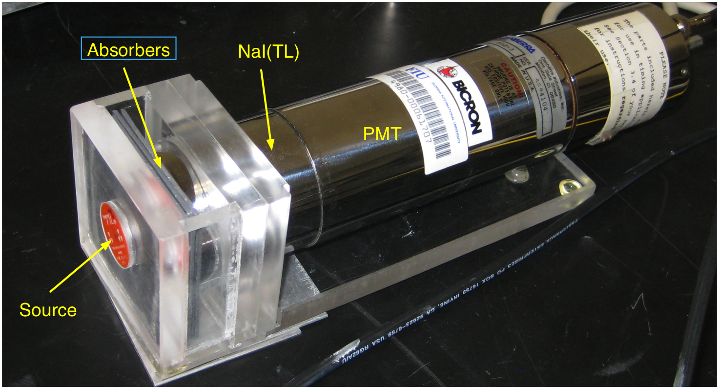
Fig. 12.1 Figure 1: Detector holder with source and absorbers

Calibrate the MCA using the \(^{137}Cs\) and the \(^{60}Co\) sources. Remember to save the spectra as ASCII (SPE) files so that you can read them using the LabTools package.

Place the \(^{60}Co\) source and the detector in the Lucite holder. Use the Preset menu to set the acquisition time to 60 second. Take data and save the spectrum. Repeat with 1, 2, …, 8 sheets of lead between the source and detector, remembering to clear the buffer between each measurement. Repeat with the sheets of aluminum. Measure the thickness of both lead and aluminum sheets.

Do the same measurements for \(^{137}Cs\) and \(^{133}Ba\).

12.3. Analysis

In each spectrum taken for the three isotopes \(^{60}Co\), \(^{137}Cs\) and \(^{133}Ba\), sum the counts under well defined photo-peaks for each setting (number of absorbing plates) and divide by the corresponding live time to obtain the rate \(R\).

For lead plot \(R\) as a function of the number of absorbing sheets and, for both lead and aluminum, plot \(ln(R)\) as a function of \(x\), the density thickness. (Density of lead \(= 11.3 g/cm^3\) ; density of aluminum \(= 2.7 g/cm^3\).) By fitting your data appropriately, determine the the total mass absorption coefficients for these materials for 1.33 MeV \(\gamma-\) rays. Also obtain the half-value layers.

Plot the obtained absorption coefficients for each material as a function of energy. What can you conclude from the energy dependence?

Do not forget the errors in your graphs and the error analysis!

12.3.1. Analysis Hints

12.3.1.1. How to sum bins in a histogram

For each spectrum add the counts in the peak. As this is a simple spectrum with only one peak, you can basically just add all channels (or bins) above a certain value. For the example you could add the channels between 400 and 1000. Assuming the spectrum is called sp when you load it, you get this sum with the command:

C, dC = sp.sum(400, 1000) # sum the channels between 400 and 1000
C, dC = sp.sum(200) # sum all channels above 200

Here C is the sum and dC is the uncertainty in the sum.

12.3.1.2. How to get the live time of a spectrum

The live time is stored in the title of the spectrum. The function below allows you to extract the number from the title:

# get the live time from a spectrum
def get_time(sp):
    tt = float(sp.title.split('=')[1].split('s')[0])
    return tt
#

Put this in your analysis script and you can get the time by doing:

t = get_time(sp)   # get the time
R = C/t            # calculate the rate
dR = dC/t          # calculate the error in the rate