11. The Franck-Hertz Experiment

11.1. Overview

The Franck-Hertz experiment, first performed in 1914, verifies that the atomic electron energy states are quantized by observing maxima and minima in the transmission of electrons through mercury vapor. The variation in electron current is caused by inelastic electron scattering which excites the atomic electrons of mercury. The Franck-Hertz tube, which contains mercury vapor, together with the electrical connections is shown in Fig. 11.1

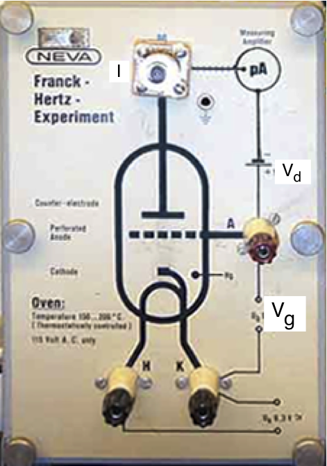
Fig. 11.1 The Franck-Hertz Tube

The reactions occurring inside the tube are described below and illustrated in Fig. 11.2 Thermionically emitted electrons from the heated cathode are accelerated towards the grid by a variable voltage \(V_{acc}\). Electrons crossing the grid are then slowed down by a \(V_{bias} \approx 1.5 V\) decelerating potential on their way towards the anode. This wat only electrons with a minimal kinetic energy of about 1.5eV will be detected. The small anode current (\(\approx 10^{-12} A\) ) has to be amplified before being measured.

If there are no mercury atoms in the tube, a small current would be observed when the accelerating voltage exceeds the the bias voltage \(V_{bias}\) and would steadily increase with increasing accelerating voltage. With mercury atoms in the tube, when the accelerating voltage, \(V_{acc}\) , is increased from zero, again a current is first observed when \(V_{acc}\) exceeds the bias voltage \(V_{bias}\) (Fig. 11.2 (a)). The current then increases with \(V_{acc}\) up to a certain threshold voltage, \(V_{th}\) , at which point the current drops sharply. The reason for this is that the kinetic energy, \(K_e = eV_{th}\), acquired by an electron matches the energy difference (4.86 eV) between the ground state (\(^1S_0\)) and an excited state (\(^3P_1\)) of the mercury atom. If it collides with an atom, it will do so in-elastically, losing kinetic energy in the process so that it can no longer overcome the 1.5V decelerating potential hill (Fig. 11.2 (b)). At lower kinetic energies, the electron collisions are elastic and no kinetic energy is lost. As \(V_{acc}\) is further increased from \(V_{th}\) , the current again starts to rise (Fig. 11.2 (c)) until it reaches a value of 2\(V_{th}\) when it drops sharply again (Fig. 11.2 (d)). Now the electron has undergone 2 sequential inelastic collisions. Thus drops in the current are observed when \(V_g = n V_{th}\) with \(n = 1, 2, 3, ...\). Note that at higher values of \(V_{acc}\) it is also possible that mercury atoms are excited to higher levels. When the current suddenly increases dramatically electrons are ejected and the mercury atoms are ionized. You can observe this effect when the mercury vapor starts glowing (have a look inside from the side).

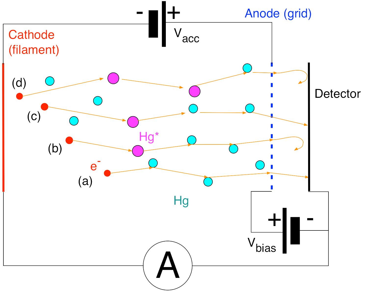
Fig. 11.2 Processes inside the Franck-Hertz tube.

11.2. Experimental Procedure

The experiment is performed with the Franck-Hertz tube inside an oven. The oven temperature controls the density of the mercury vapor inside the tube and thus influences the frequency of collisions between electrons and mercury atoms. The pressure of the mercury vapor is its vapor pressure. If you do not know what vapor pressure is, read up on it as it is an important quantity.

DO NOT SWITCH ANYTHING ON UNTIL YOUR CIRCUITS HAVE BEEN CHECKED BY THE INSTRUCTOR.

Connect the Control Unit to the Franck-Hertz tube as shown in Fig. 11.3. This is straightforward since the various outputs are clearly labeled with the letters M, A, K, and H which also appear on the Franck-Hertz tube oven unit. (The “control grid” output for a neon tube is not used.)

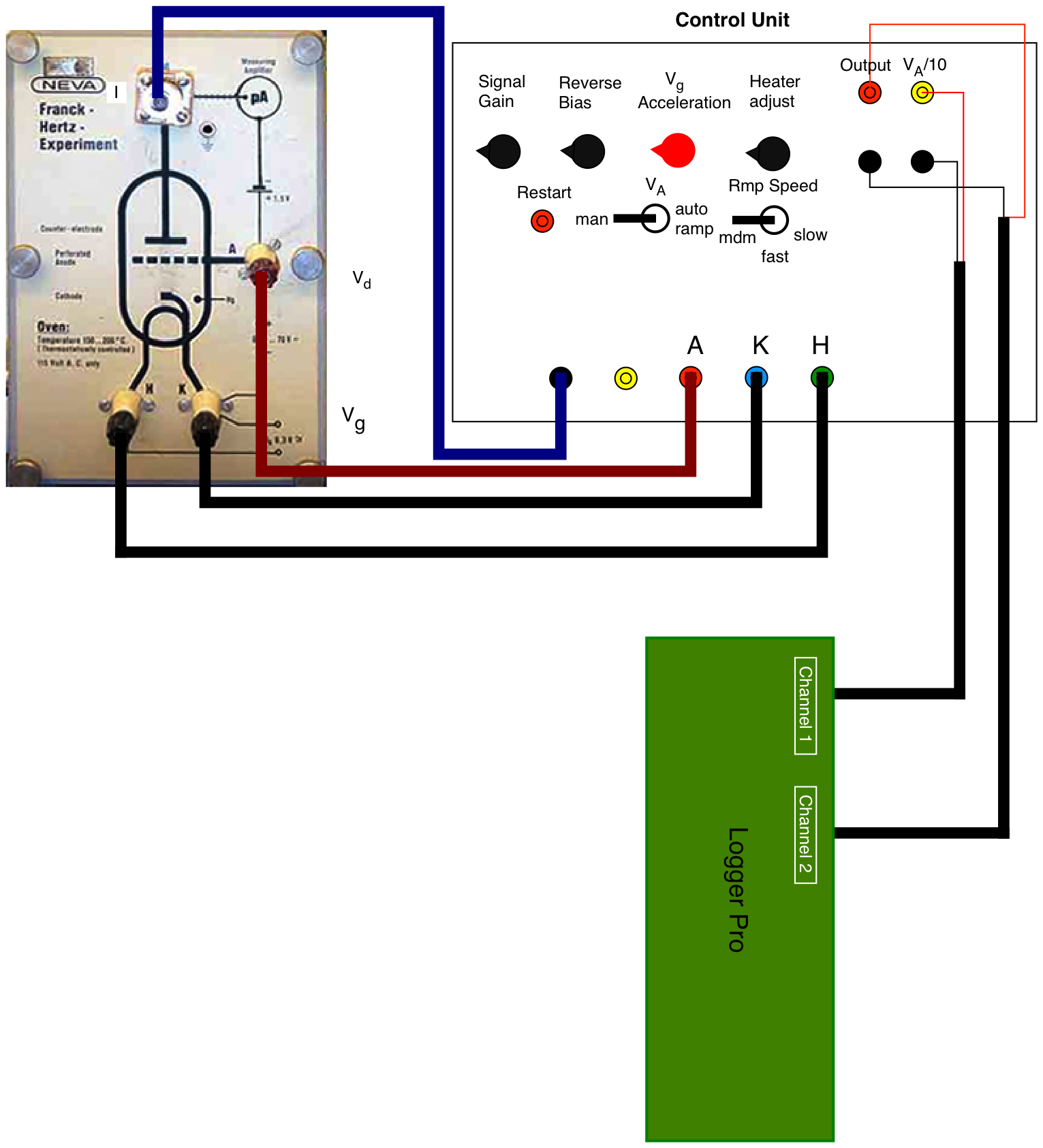
Fig. 11.3 Setup of the Franck-Hertz experiment

Connect the Logger Pro unit via USB to the Mac. Connect the two voltage probes to channel 1 and 2. Connect the probe tips of channel 1 to the output that is proportional to \(V_{acc}\) as show in Fig. 11.3. Connect the other probe tips to the signal output as shown in the figure. On the Mac start the Logger Pro program. Load the configuration FH_experiment from the Desktop. This configures Logger Pro for this experiment.

(Ask your Instructor to help you with the setup if there are problems).

Turn on the temperature controller and set the oven temperature to 340^oF.Wait for about 15 minutes for the temperature to stabilize. Turn the Heater adjust control to give a filament voltage between 5.0 and 5.5 V. Set the Reverse Bias voltage control halfway between the first and secondmark at around the 7 o’clock position. This provides the ~1.5 V decelerating potential between the grid and anode. Set the gain to about the 3rd mark. Set the \(V_{A}\) control to manu and press the reset button.

Now you are ready to take data.

1. Switch the \(V_{A}\) control to auto ramp, and press the restart button, after a few seconds delay the accelerating voltage \(V_{acc}\) will start to ramp up automatically

2. Start the data collection and observe the data being taken.

3. if the signal jumps, becomes erratic or the ramping stops, stop the data collection, press the restart button and switch from auto ramp to manu manual.

4. Export the data to as csv file.

Repeat this procedure a few times, adjust signal gain and bias voltage for an optimal signal response. Repeat these measurements for T = 400, 450 and 500 ^oF. From the data determine the energy difference between the ground state (\(^1S_0\)) and the excited state (\(^3P_1\)). Does the energy difference between the various peaks confirm that several inelastic collisions occurred or du they suggest that in a single collision the mercury atom is excited to higher states.

11.3. Analysis Hint

11.3.1. Convert CSV files to data files

To analyze the data using the Python LabTools, download the python script csv2data.py and run it in ipython:

run csv2data.py my_logger_file.cvs

This will convert the csv file you created to a standard data file (for the example above it would be my_logger_file.data) that you can read with B.get_file.

11.3.2. Determine peak positions

To determine the peak locations as precisely as possible fit the peak part of the data with a parabola (using B.polyfit). Careful, you should only fit that part of a peak that looks similar to a parabola. You can do this by selecting only the subset of the data points surrounding the peak.

To find the limits around the peak use the zoom tool and plot only the top of the peak. Make sure that your x-axis limits determine the selected part of the peak. Once your peak is selected type:

xlim()

and the function will return a pair of numbers (xmin, xmax) corresponding to the current x-axis limits of your plot. You can then copy and pase these into your analysis script or a data file to determine your peak limits for fitting.

Using these number you can select the corresponding subset of your data as follows:

w = (xmin <= x) & (x <= xmax) # or
w = B.in_window(xmin, xmax, x)

this returns an array (full of True and False values) with the information on which part of x satisfies the condition \(xmin \leq x \leq xmax\). To fit only those values that satisfy your selection you do:

f = B.polyfit( vg[w], s[w] )

where vg is the array containing the accelerating voltage values and s is the signal array. When polyfit is used as shown above, you are fitting a parabola

(11.1)\[S = a_0 + a_1 V_g + a_2 V_g^2\]

where the \(a_j\) are the fit parameters with the correspondence \(a_j = f.par[j], j = 0,1,2\). From the knowledge of the \(a_j\) you can calculate the position of the maximum (derive this expression as an exercise). Ask your instructor on how to calculate the uncertainty in the position of the maximum. To obtain the best estimate, you need to use the covariance matrix. (see Estimating Measurement Errors)

From these peak positions you can determine the energy difference between the ground and the excited state of Mercury. Make a plot of the energy difference as a function of peak position for the different temperatures. What is the average value and its uncertainty? Discuss your result.