1. Summary of Error Analysis and Statistical Methods

1.1. Overview

There are two main types of experiments in physics:

1. One tries to determine some physical quantity with the highest precision possible e.g. the speed of light, the elementary charge, the gravitational constant etc. In other words the experiments goal is to determine some parameters.

2. The goal of the other type of experiment is to test whether a particular theory or theoretical model agrees with experiment. These type pf experiments test a hypothesis.

Very often these two experiment types have a large overlap. Most experiments carried out in intermediate lab is of the first type where you have to determine a physical quantity with the highest accuracy and precision possible. This quantity e.g. Planck’s constant is determined from various other directly quantities such as voltages, currents, distances etc. When you perform the same measurement repeatedly you will observe that you will get slightly different results from which you can determine an average value. We are assuming that the experimental conditions are completely reproducible in such a way that by repeating the same measurement an infinite number of times you would obtain the true value with infinite precision and accuracy. In reality this is not possible and you need to estimate the true value from the existing measurements, together with a good estimate of the range of values within which you expect the true value to lie. This last quantity you can call the experimental uncertainty or error or precision. How you obtain these best estimates from a finite number of measurements is the subject of statistics and error analysis.

There are many excellent books on statistics and error analysis in experimental physics (a classical book is Data Reduction and Error Analysis for the Physical Sciences 3rd Edition,by Philip Bevington and D. Keith Robinson, or An Introduction to Error Analysis: The Study of Uncertainties in Physical Measurements by John R. Taylor. Another more advanced book : Statistical Methods in Experimental Physics: 2nd Edition by Frederick James) which discuss measurement errors and uncertainties and how statistical methods can be used to obtain best estimates on quantities extracted from measurements. The following sections are basically a very short summary of the main results developed in these books. You should use these techniques to analyze your data to obtain reasonable estimates for your measurement values and their uncertainties.

1.2. Accuracy vs Precision

There is a difference between what one means with accuracy and precision. The accuracy is a measure of how close the experimental value is to the true one. The precision determined how reproducible your experimental value is. It is often useful to determine the relative precision where the uncertainty of your result is expressed as a fraction of the value of the result. A good experiment needs to consider accuracy and precision simultaneously. An experiment can be very precisie but if e.g. the calibration of your instrument is wrong then your result will be inaccurate. While an imprecise experiment might be accurate but you are not going to learn anything new from it.

If you have an experimental result where you determined e.g. Planck’s constant, in the discussion of the results you should compare the accuracy of your result (how much it deviates from the currently accepted much more precise value) compared to the precision of your result. If the published value lies within your estimated uncertainty then you can be happy as your experiment agrees within its precision. If not, you need to try to understand what is going on, did you discover new physics or was there something else that lead to the results that contributed to the deviation or is your estimate of the precision of your result overly optimistic ?

1.3. Notation: Significant Figures and Roundoff

The precision of an experimental value is indicated by the number of digits used to represent the results including the uncertainty of the result. Here are the rules regarding significant figures when you use scientific notation (\(1234 = 1.234\cdot10^3\))

1. The leftmost non-zero digit is the most significant one

2. The rightmost digit is the least significant one

3. All digits between the least and the most significant digits are counted as significant digits or significant figures.

4. When quoting an experimental result the number of significant figures should be approximately 1 more than that dictated by the experimental precision to avoid rounding errors in later calculations. E.g. you determined the elementary charge to be \(1.624\pm\ 10^{-19}\ C\) with an uncertainty of \(2.5\ 10^{-21}\ C\) then you would quote that result as \(Q = (1.624\ \pm 0.025)\cdot 10^{-19}\ C\).

5. If you have a large uncertainty in the above example e.g. \(8.7\ 10^{-21}\ C\) the you would quote the result as \(Q = (1.62\ \pm 0.09)\cdot 10^{-19}\ C\). You let the uncertainty define the precision to which you quote the result.

When your drop insignificant figures the last digit retained should be rounded according to the following rule (the computer can do this for you):

1. If the fraction is larger that 0.5 increment the new least significant digit.

2. If the fraction is less than 0.5 do not increment

3. If the fraction is equal 0.5 increment the new least significant digit only of it is odd.

Examples: 1.234 is rounded to 1.23, 1.236 is rounded to 1.24, 1.235 is rounded to 1.24 and 1.225 is rounded to 1.22

1.4. Types of Errors/Uncertainties

There are two main type of errors which can have a variety of reasons:

1. Random errors: these are due to fluctuations of observations that lead to different results each time the experiment is repeated. They require repeated measurements in order to achieve a precision which corresponds to the desired accuracy of the experiment. Random errors can only be reduced by improving the experimental method and refining the experiment techniques employed. Random errors can be due to instrumental limitations which can be reduced by using better instruments or due to inherent limitation of the measurement technique. For example, if you count the number of random processes occurring during a time intervall, if the time intervall is too short and the total number of counts too small the relative precision will be limited, even though you might have the best instrument available.

2. Systematic Errors: this type of error is responsible for the deviation of even the most precise measurement from the tru value. These errors can be very difficult to determine and a large part of designing and analyzing an experiment is spent on reducing and determining its systematic error.

1.5. Estimating Measurement Errors

There are two important indices of the uncertainty in a measured quantity, the maximum error and the standard error (note these names can be different in different books).

Maximum error: This is supposed to indicate the range within which the true value definitely lies. With a single measurement, it is really the only type of error that can be estimated.

Standard error: If you have a large number \(N\) of measurements of a single quantity, \(t\), will produce a “normal” or “Gaussian” distribution curve as shown below. The ordinate, \(n(t)\), is the number of observations per unit range of \(t\) whose values lie between \(t\) and \(t+dt\). The equation for the curve is:

(1.1)\[n(t) = \frac{N}{\sigma\sqrt{2\pi}} e^{-(t - \bar t)^2/2\sigma^2}\]

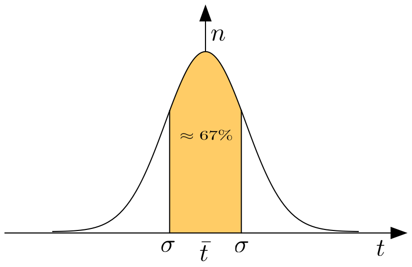
Fig. 1.1 Gaussian distribution curve.

This curve is symmetrical about the mean value, \(\bar t\). \(N\) is the total number of observations, and \(\sigma\) is a measure of the width of the curve and is called the standard deviation or standard error. For this distribution \(\sigma\) is the RMS value of the departures of the individual \(t\) measurements from the mean, \(\bar t\). The square of the RMS value is also the so-called variance of \(t\):

(1.2)\[\sigma_t^2 = \frac{1}{N}\sum_i (t_i - \bar t)^2\]

You can verify that 67% of all measurements of \(t\) lie within \(\bar t \pm \sigma\), 95% within \(\bar t \pm 2\sigma\) and 99.7 % within \(\bar t \pm 3\sigma\). In reality \(\bar t\) and \(\sigma\) are not known and need to be estimated from the data.

An important application is the estimate of the uncertainty of a counting experiment where the number of randomly occurring events are counted during a certain time intervall (e.g. particle emitted by a radioactive source):

Lets assume you have a single measurement with the result, \(N_{exp}\) counts. One assumes now that \(N_{exp}\) represents the mean for this measurement that you would obtain if you repeated this it many times, but which you actually do not do. This is of course a rather coarse approximation but the only one possible. In that case the estimate of the standard deviation for this measurement would be \(\sigma_{N} = \sqrt{N_{exp}}\), a really important result which is widely applied.

1.6. Combination of Errors

1.6.1. Independent Quantities

The discussion in this section is what you will use most of the time when you perform the error analysis of your data.

Usually in an experiment, the final result is derived from a number of measured, and usually independent quantities, \(x, y, z, ...\), connected to the required quantity, F, by some mathematical formula. It is therefore necessary to determine how errors/uncertainties in the measured quantities affect the final result.

In general, if \(F = f(x, y, z, .......)\), then we can estimate the maximal error by:

(1.3)\[\delta F = \left\vert\frac{\partial F}{\partial x}\right\vert\delta x + \left\vert\frac{\partial F}{\partial y}\right\vert\delta y + \left\vert\frac{\partial F}{\partial z}\right\vert\delta z + ...\]

where \(\delta x\) is the maximal error of the quantity \(x\).

We can determine the standard error \(\sigma_F\) using the following expression:

(1.4)\[\sigma_F = \sqrt{\left(\frac{\partial F}{\partial x}\right)^2\sigma_x^2 + \left(\frac{\partial F}{\partial y}\right)^2\sigma_y^2 + \left(\frac{\partial F}{\partial z}\right)^2\sigma_z^2 + ...}\]

This assumes that all quantities \(x,y,z,...\) are independent of each other. Typically you will quote the standard error.

1.6.2. Dependent Quantities, Covariance

The error analysis of data with measurements that are possibly correlated is a bit more complex than the previous examples and is illustrated using a simple example.

We will first consider a new quantity \(y_i = a x_{i1} + b x_{i2}\) which is linear combination of two experimental quantities \(x_{i1}, x_{i2}\) that are determined during measurement \(i\) of a total of \(N\) experiments, hence \(i = 1,2,3...,N\). First we can calculate the mean:

\begin{eqnarray*} \bar y & = & \frac{1}{N}\sum_{i=1}^N y_i \\ & = & \frac{1}{N}\sum_{i=1}^N (a x_{i1} + b x_{i2}) \\ & = & a\bar x_1 + b \bar x_2 \\ \end{eqnarray*}

Next we can calculate the variance of \(y\):

\begin{eqnarray*} \sigma_y^2 & = & \frac{1}{N}\sum_{i=1}^N (y_i - \bar y)^2 \\ & = & \frac{1}{N}\sum_{i=1}^N \left( (a x_{i1} + b x_{i2}) -(a\bar x_1 + b \bar x_2)\right)^2 \\ & = & \frac{1}{N}\sum_{i=1}^N \left(a^2(x_{i1} - \bar x_1)^2 + b^2(x_{i} - \bar x_2)^2 + 2ab(x_{i1}- \bar x_1)(x_{i2} - \bar x_2)^2\right) \\ & = & a^2 \sigma_1^2 + b^2 \sigma_2^2 + 2ab\ cov(x_1, x_2) \\ \end{eqnarray*}

where \(cov(x_1,x_2) = \frac{1}{N}\sum_{i=1}^N \left((x_{i1}- \bar x_1)(x_{i2} - \bar x_2)\right)\) is the covariance of \(x_1\) and \(x_2\). It is a measure of the correlation between the two variables and can be positive, negative or zero. If \(x_1\) and \(x_2\) are completely independent of each other their covariance is 0. This is a simple example of a linear function of measured quantities which can be generalized to the general function \(F = f(x_1, x_2, x_3, ..., x_n)\) as follows:

(1.7)\[\sigma_F^2 = \sum_{i= 1}^n \left(\frac{\partial F}{\partial x_i}\right)^2\sigma_{x_i}^2 + \sum_{i\neq j= 1}^n \frac{\partial F}{\partial x_i} \frac{\partial F}{\partial x_j} cov(x_i,x_j)\]

(1.8)\[\sigma_F^2 = \sum_{i,j = 1}^n \frac{\partial F}{\partial x_i} \frac{\partial F}{\partial x_j} cov(x_i,x_j)\]

1.6.3. Examples

Here a a few examples of how to practically apply the above expressions. They are taken from the analysis of experiments that you are analyzing:

1. You have measured an angle \(\theta \pm \sigma_\theta\) e.g. in a spectroscope where \(\theta = \theta_{deg}, \theta_{min}\) is in degrees(\(\theta_{deg}\)) and minutes(\(\theta_{min})\) and \(\sigma_\theta\) is in minutes. During your analysis you need to calculate the cosine of this angle and need to know the error in the cosine. How to you proceed?

   • Convert the degrees and minutes to radians: \(\theta_r = \frac{\pi}{180}\left(\theta_{deg} + \frac{\theta_{min}}{60}\right)\), \(\sigma_{\theta_r} = \frac{\pi}{180}\left(\frac{\sigma_{\theta}}{60}\right)\)

   • Apply (1.3) where \(f\) is \(\cos{\theta}\) and x is \(\theta\) and no other variables.

   • The result should be \(\sigma_{\cos} = \sqrt{ \left( \frac{d\cos}{d\theta}\right) ^2 \sigma_r^2 } = \sin{\theta_r}\sigma_r\)

2. You encounter a problem where you need to estimate the uncertainty of a quantity that contains the square root of an experimentally determined count rate \(R = N/\Delta t\) where \(N\) is the number of counts observed in the time \(\Delta t\). Assuming an uncertainty of \(\sigma_t\) for the time interval what is the uncertainty of \(\sqrt{R}\)?

   • Calculate the uncertainty of \(N\) using the fact that it is the result of a counting experiment: \(\sigma_N = \sqrt{N}\).

   • We need therefore to determine the uncertainty of the function \(f(N, {\Delta t}) = \sqrt{\frac{N}{\Delta t}}\)

   • This is a function of 2 variables (\(N\) and \(\Delta t\)) so you need to calculate the corresponding partial derivatives according to equation (1.3) as follows:

   • \(\frac{df}{dN} = \frac{1}{2\sqrt{N \Delta t}}\) and \(\frac{df}{d\Delta t} = \frac{-1\sqrt{N}}{2\sqrt{\Delta t^3}}\)

   • Combining the derivatives and uncertainties you get:

     \(\sigma_f = \sqrt{\left(\frac{1}{2\sqrt{N \Delta t}} \right)^2 N + \left(\frac{-1\sqrt{N}}{2\sqrt{\Delta t^3}}\right)^2 \sigma_t^2}\)

   This a bit more complex but basically the same procedure as before.

3. This example shows how to use the covariance matrix that is returned by every fit. This matrix contains information on the correlation between fit parameters. The simple error propagation (1.3) is only valid if the quantities \(x, y, z\) are independent from each other. When these quantities are fit parameters, e.g. the slope and offset of a line, or the parameters of a polynomial, they are most likely not independent. In this case you need to take into account their correlation as described in (1.8).

   As an example we try to determine the location of a peak and its uncertainty:

   • Start by fitting the data points around the the top of the peak with a parabola (in this way we approximate the top part of the peak with a parabola) \(y = a_0 + a_1 x + a_2 x^2\)

   • Determine the location of the maximum \(x_m\) by solving: \(\left. \frac{dy}{dx}\right|_{x_m} = 0\), resulting in \(x_m = -\frac{a_1}{2a_2}\). The determined peak position is now a function of 2 variables \(x_m(a_1, a_2)\).

   • These fit parameters also have their own errors \(\sigma_{a_1}, \sigma_{a_2}\) which are NOT independent and we need to use equation (1.8):

   • First we calculate the two partial derivatives \(\frac{\partial x_m}{\partial a_1} = \frac{1}{2 a_2}\) and \(\frac{\partial x_m}{\partial a_2} = -\frac{a_1}{2 a_2^2}\). Since \(x_m\) is independent of \(a_0\) all its partial derivatives are 0.

   • Using eq. (1.8) we get therefore:

     \(\sigma_{x_m}^2 = C_{11}\left(\frac{\partial x_m}{\partial a_1}\right) ^2 + 2C_{12}\left(\frac{\partial x_m}{\partial a_1}\right)\left(\frac{\partial x_m}{\partial a_2}\right) + C_{22}\left(\frac{\partial x_m}{\partial a_2}\right) ^2\)

     Where the \(C_{ij}\) are the covariance matrix elements :cov[i,j]. Inserting the expressions for the derivatives results in:

     \(\sigma_{x_m}^2 = C_{11}\left(\frac{1}{2 a_2}\right) ^2 - 2C_{12}\left(\frac{1}{2 a_2}\right)\left(\frac{a_1}{2 a_2^2}\right) + C_{22}\left(\frac{a_1}{2 a_2^2}\right) ^2\)

     This is a similar expression as eq. (1.3) since \(C_{ii} = \sigma_{a_i}^2\) but with an additional term that can be negative. The final correlated error can therefore be smaller than the one obtained from (1.3) for quantities that are correlated.

1.7. Mean, Least Squares

Assume that you have measured a set of \(N\) data points of the same quantity \(x\). These represent a finite, random selection from an imaginary population of an infinite number of data points, distributed according to e.g. a Gaussian distribution function, characterized by the mean, \(\mu\) , and the variance \(\sigma\). The probability of observing a value \(x_i\) for the \(i^{th}\) data point is then:

(1.9)\[P_i(x_i, \mu, \sigma) = \frac{1}{\sigma\sqrt{2\pi}}\exp{\left[ -\frac{1}{2}\left(\frac{x_i - \mu}{\sigma}\right)^2\right]}\]

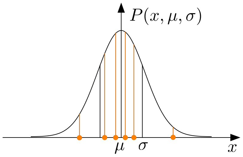
Fig. 1.2 A sample \(x_1, x_2, ...\) and its distribution curve.

In reality we do not know the true mean for a distribution but have to estimate it. The question then is what is the best method to approximate the true mean given only a finite set of data points. If we know the the data are distributed according a gaussian with a certain \(\sigma\) we can determine the total probability or likelihood to observe the given set of data points assuming a value \(\mu'\) for the mean.

(1.10)\[P_{tot}(\mu') = \prod_{i=0}^N P_i(x_i, \mu', \sigma) = \left(\frac{1}{\sigma\sqrt{2\pi}}\right)^N\exp{\left[ -\frac{1}{2}\sum_{i=0}^N\left(\frac{x_i - \mu'}{\sigma}\right)^2\right]}\]

The best value for \(\mu'\) is the one for which \(P_{tot}\) is a maximum. This is an example of the method of maximum likelihood. In order for \(P_{tot}\) to be maximal the expression:

(1.11)\[X = -\frac{1}{2}\sum_{i=0}^N\left(\frac{x_i - \mu'}{\sigma}\right)^2\]

needs to be minimal and therefore \(\partial X/\partial \mu' = 0.\) This leads then to the expected result:

\begin{eqnarray*} \mu' & = & \frac{1}{N}\sum_{i=1}^N x_i \\ \sigma_{\mu'}^2 & = & \frac{\sigma}{N}, \text{ where} \\ \sigma^2 = s^2 & = & \frac{1}{N-1}\sum_{i=1}^N (x_i-\bar x)^2 \end {eqnarray*}

Here \(\sigma_{\mu'}\) is the standard error of the mean calculated using error propagation as outlined (1.4), and \(\sigma\) has been estimated from the data as shown above.

If each data point has a different error, one has to assume that the set of measurements is a sample drawn from a set of different distributions with the same mean but different \(\sigma's\). In that case the maximal likelihood is obtained by minimizing

(1.13)\[X = -\frac{1}{2}\sum_{i=01}^N\left(\frac{x_i - \mu'}{\sigma_i}\right)^2\]

which leads to the definition of the so-called weighted mean:

\begin{eqnarray*} \mu' & = & \frac{\sum_{i=1}^N \left( x_i/\sigma_i^2 \right)} {\sum_{i=1}^N \left( 1/\sigma_i^2\right) } \\ \sigma_{\mu'}^2 & = & \frac{1}{\sum_{i=1}^N \left( 1/\sigma_i^2 \right)} \\ \end {eqnarray*}

1.8. Least Square Fitting, Parameter Determination

In the introduction of this chapter the two main type of experiments were listed as parameter determination and hypothesis testing. Both of these often lead to the problem that you have measured a quantity \(y_i\) that depends on another measured quantity \(x_i\). Let’s assume that the experimental uncertainty \(\sigma_{y_i} \ll \sigma_{x_i}\) and that \(\sigma_{x_i}\) can be neglected. In that case we can assume that the set of experimental \(y_i\)-values represents a random sample of data drawn from distributions centered around a value of \(y(x_i)\) with a width of \(\sigma_i\). The determination of the function \(y = f(x_i)\) can now be either the subject of parameter determination, of hypothesis testing or a combination of both. For parameter determination, we further assume that one can write \(y(x_i) = f(x_i, a_0, a_1, ..., a_n)\) where \(a_i\) are parameters that need to be determined from the experimental data and the goal of the fitting process is the determination of the best set of parameters that reproduce the experimental data set.

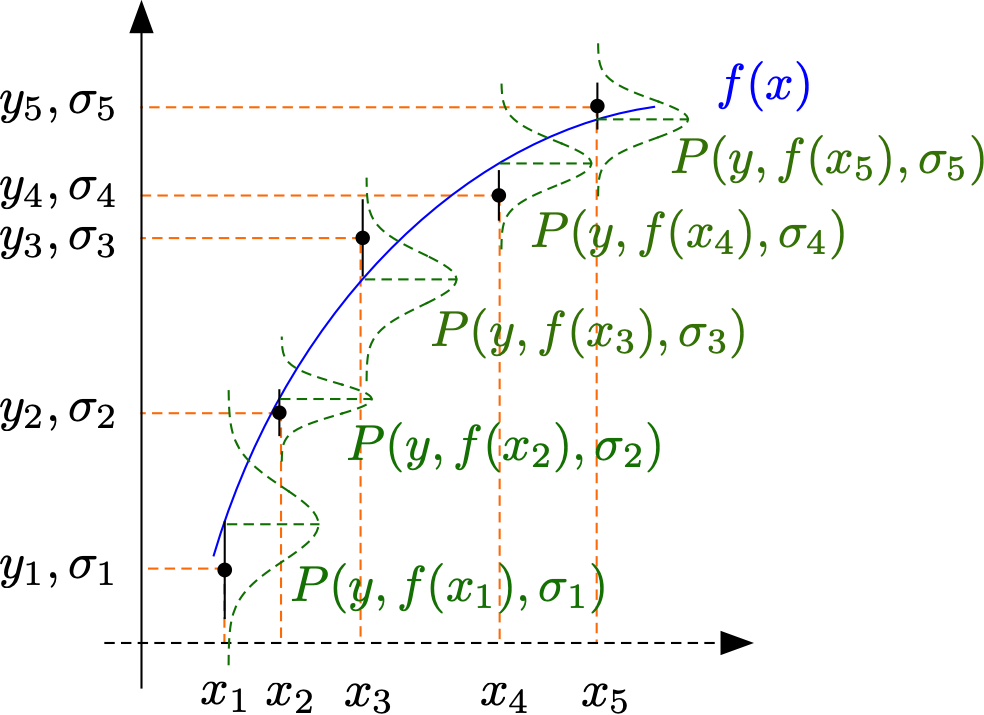
Fig. 1.3 Experimental points \((x_1,y_1), (x_2,y_2) ...\), together with their distribution functions from which they were drawn and the function \(f(x)\) which should be estimated from the data.

In order to determine the parameters \(a_0, a_1, ..., a_n\) one maximizes the total likelihood for obtaining the observed set of data \((x_i, y_i, \sigma_i)\) with respect to these parameters .

(1.15)\[P(a_0, a_1, ... , a_n) = \prod_{i=1} \left[\frac{1}{\sigma_i\sqrt{2\pi}}\right]\exp{\left[ -\frac{1}{2}\left(\frac{y_i - f(x_i, a_0, a_1, ...)}{\sigma_i}\right)^2\right]}\]

Maximizing \(P(a_0, a_1, ... , a_n)\) corresponds to minimizing the quantity \(\chi^2\):

\begin{eqnarray*} \chi^2 & = & \sum_{i=1}^N\left(\frac{y_i - f(x_i, a_0, a_1, ...)}{\sigma_i}\right)^2 \\ \frac{\partial \chi^2} {\partial a_i}& = & 0\ \text{for } i = 1, ... , n \\ \end{eqnarray*}

This forms the basis of least square fitting. Different fit algorithms have been developed depending on whether the fit function is linear in the parameters (linear fit) or non linear. They differ in the method of finding the minimum but all return the parameters at the minimum together with their variances (standard errors) and their covariances in form of the so-called covariance matrix. All fitting routines will return the quantity \(\chi^2\) and \(\chi^2_\nu = \chi^2/\nu\) where \(\nu = N - n\) the number of degrees of freedom of the fit. \(\chi^2_\nu\) is also called the reduced \(\chi^2\). Since a data set is considered a random sample the value of \(\chi^2\) is also a random variable following its own distribution function:

(1.17)\[P(x^2,\nu) = \frac{(x^2)^{\frac{1}{2(\nu-2)}} e^{-\frac{x^2}{2}}}{2^{\frac{\nu}{2}}\Gamma(\nu/2)}\]

This can be used to either have a measure of the quality of the fit and/or how well the chosen fitting function \(f(x_i, a_0, a_1, ..., a_n)\) represents the true functional relationship \(y(x)\). The latter is an important part of hypothesis testing. Since a distribution function does not give a probability for a specific value of \(\chi^2_\nu\) but a probability density, one chooses an integral over the distribution function as a measure for the quality of a fit (also called the goodness of a fit) or a test of a hypothesis:

(1.18)\[P(\chi^2,\nu) = \int_{\chi^2}^\infty P_x(x^2, \nu) dx^2\]

Here \(P(\chi^2,\nu)\) is the probability that another random set of \(N\) data points drawn from the same parent distribution would yield an equal or larger value of \(\chi^2\) than the one obtained.

For a fitting function that is a good approximation to the true function and with realistic error estimates one should obtain an average \(\chi^2\)-value for which \(P(\chi^2,\nu)\approx 0.5\). A poorer fit will produce a larger value of \(\chi^2_\nu\) with a much smaller value of \(P(\chi^2,\nu)\). In general fits with \(P(\chi^2,\nu)\) reasonably cose to 0.5 have a reduced \(\chi^2_\nu \approx 1\) or typically < 1.5.

The interpretation of \(\chi^2_\nu\) is always somewhat ambiguous as it depends on the quality of the data as well as on the choice of the fitting function.

In general, fitting a function which is non-linear in the parameters is more challenging as reasonable initial values need to be assigned to the fit parameters. Also if a minimum in \(\chi^2_\nu\) has been found it is not necessarily a global minimum. Therefore the parameters and the value of \(\chi^2_\nu\) need to be studied. If parameters are highly correlated it is also possible that a fit fails, i.e. a matrix cannot be inverted and a minimum cannot be found, this is usually a sign of an ill posed problem.