9. The e/m Ratio
9.1. Background
This classic experiment was first carried out by J.J.Thomson in 1897. It involves the use of an electric field to accelerate electrons up to high velocity, and a magnetic field to then steer the electrons in a circular trajectory. The electrons are released by thermionic emission from a heated filament (cathode) and are accelerated towards a cylindrical anode. See Fig.1 and Fig.2. This is a similar situation to the electron gun used to generate the electron beam in an X-ray tube or in an electron microscope
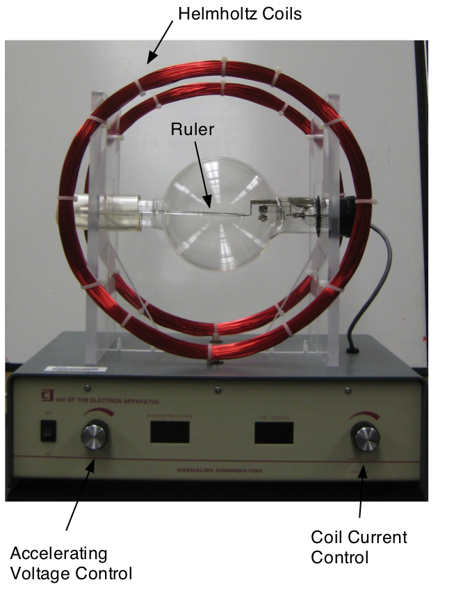
Fig. 9.1 Picture of the e/m apparatus.
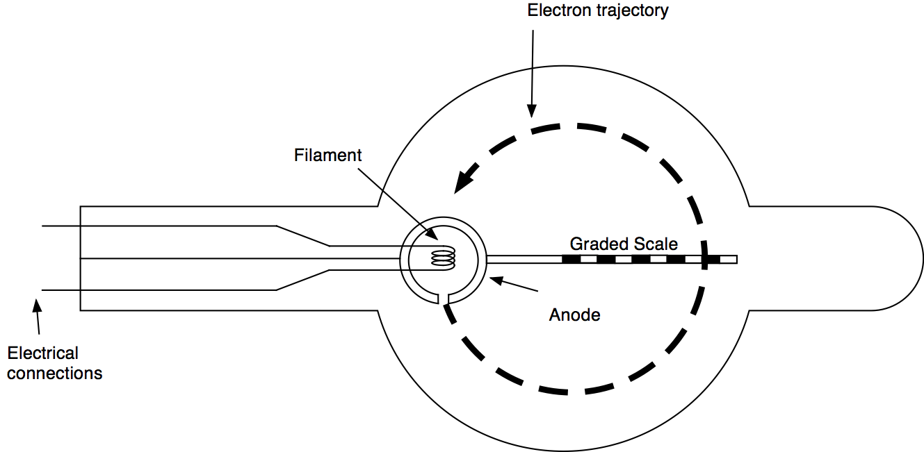
Fig. 9.2 Schematic of the e/m apparatus.
As the electrons accelerate from the cathode to the anode, they loose potential energy, \(U_e = e V\) (\(V\) is the accelerating potential and \(e\) is the elementary charge), and gain an equal amount of kinetic energy, \(K_e = \frac{1}{2}m_e v^2\) ( \(m_e\) is the electron mass and \(v\) the electron velocity) . Therefore they arrive at the anode with a velocity given by:
Some of the electrons escape with this velocity though a narrow aperture in the anode into a region where a uniform magnetic field (\(\vec{B}\)) exists. In Fig. 9.1 this field, which is not shown would point out of of the paper and towards the reader. The field exerts a magnetic force (\(\vec{F}\) ) with a magnitude of \(F = evB\) (since the velocity and the magnetic field are perpendicular to each other). The direction of the force is perpendicular to the velocity and acts as a centripetal force:
where \(r\) is the radius of the path. Eliminating \(V\) between equations (9.1) and (9.2) one obtains the charge to mass ratio:
The magnetic field is produced by the current flowing in two Helmholtz coils. The distance between these circular coils is equal to their radius, an arrangement that results in a reasonably uniform, axial magnetic field midway between the coils. The magnitude of the magnetic field, \(B\) , in this region sis given by
where
- N:
Number of turns in each coil (132)
- I:
Current
- R:
Radius of the coil
You should verify the previous derivation!
9.2. Experimental Procedure
We are going to determine the ratio \(e/m_e\) by determining the B-field and the radius of curvature of the electron beam in the magnetic field. To do this you select an accelerating voltage \(V\) and keep it constant while you vary the magnetic field by varying the current in the coils. For each magnetic field setting you will then determine the radius of curvature of the beam. From each measurement you should be able to extract the ratio \(e/m_e\) and in the end you will calculate the (weighted) average.
9.2.1. Data Taking
Select the following accelerating voltages: 200 , 250, 300 and 400 V. How well do you think you know the voltage ?
For each voltage setting record the current in the coil and the path diameter (or the radius) of the electron path. Make about 10 measurements equally spaced between the smallest and the largest current for which you can still measure the path diameter. Estimate the error of the diameter (radius) measurement. How well to you know the current ?
Record your data for each voltage setting.
Measure the diameter of the Helmholtz coils and note the number of windings.
9.2.2. Uncertainty/Errors
All measured quantities have an uncertainty associated with them as it is impossible to measure any quantity with infinite precision. An experimental uncertainty is also often called an experimental error. This should NOT be confused with the difference between a published or theoretical value and your experimental result. The experimental uncertainty is often represented by the symbol \(\sigma\). If several experimental quantities contribute to your final result you need to estimate how the uncertainties in your measurements will affect the uncertainty in your final result. The simplest estimate is to calculate the partial derivatives of your final results with respect to each experimental quantity and add the various contributions in quadrature.
Let’s assume you have measured the quantities \(x_e \pm \sigma_x, y_e \pm \sigma_y\) and \(z_e \pm \sigma_z\), where \(\sigma_x, \sigma_y, \sigma_z\) are the respective uncertainties (measurement errors). You use these values to calculate a new quantity
You can now determine the uncertainty \(\sigma_Y\) as follows:
Let’s apply this to the ratio \(R_{em} = \frac{e}{m_e} = \frac{2V}{B^2 r^2}\). Note that all variables, \(V, B, r\) have uncertainties \(\sigma_V, \sigma_B, \sigma_r\).
\(\sigma_V\), uncertainty in \(V\) from reading the instrument
\(\sigma_B\), uncertainty in \(B\) this needs to be calculated since the field is a function of \(N, R\) and \(I\) (see (9.4) which are all measured quantities that have uncertainties: \(\sigma_N,\sigma_R, \sigma_I\)
\(\sigma_r\), uncertainty in \(r\) from measuring \(r\).
9.2.2.1. Error Calculations:
First calculate \(\sigma_B\) using (9.6) and (9.4)
Next we calculate the error in \(R_{em}\) using the results of (9.7) for \(\sigma_B\) :
Derive these expressions yourself verify that they are correct.
Using these expressions you can calculate the uncertainty for each value of \(R_{em}\).
9.2.2.2. Weighted Mean:
Assume you have several experimental values \(X_i \pm \sigma_i\), where \(i = 1 ... N\), for the same quantity \(X\) (e.g. \(R_{em}\)). You want to calculate the average of these values taking into account the uncertainty associated with each individual one. This means that a measurement with a big uncertainty should not contribute as much as a measurement with a much smaller uncertainty. This can be done using the following expressions:
where \(\bar{X}\) is the weighted mean and \(\sigma_{\bar{X}}\) its uncertainty.
9.2.3. Analysis
For each data point calculate \(B\) and \(\sigma_B\)
For each data point calculate \(R_{em}\) and its uncertainty \(\sigma_{R_{em}}\).
Make a plot of \(R_{em}\) (including error) as a function of the current, \(I\), in the coil, for each data set taken at constant \(V\). \(R_{em}\) should NOT depend on \(I\)
Calculate the weighted average for \(R_{em}\) and calculate its error.