5. Black-Body Radiation

5.1. Background

A body at a certain temperature continuously absorbs and emits electromagnetic radiation. If it absorbs more energy that it emits its temperature will increase and if it emits more energy than it absorbs it’s temperature will decrease. When it is in a thermal equilibrium with its surroundings then it absorbs the same amount of power as it emits. An ideal body that absorbs all electromagnetic radiation that impinges on its surface is called a black body. The spectrum of the radiation emitted by a black body is entirely determined by its temperature and independent of its composition.

In 1900, Max Planck obtained his famous black-body formula that describes the energy density per unit wavelength interval of the electromagnetic radiation emitted by a black-body at a temperature \(T\) :

(5.1)\[u(\lambda,T) = \frac{8\pi h c}{\lambda^5(e^{hc/\lambda kT} - 1)}\]

where \(\lambda\) is the wavelength, \(T\) is the temperature of the body, \(k\) is the Boltzmann constant, \(h\) is Planck’s constant and \(c\) is the speed of light.

A good realization of a black body is a cavity with a small hole through which a small amount of radiation can exit (for observation) without disturbing the thermal equilibrium inside. If one assumes for simplicity that the cavity is made out of an electric conductor, one can show that only certain standing transverse electromagnetic waves are allowed. Each electromagnetic wave behaves statistically like a harmonic oscillator of a certain frequency. While a classical oscillator can contain any amount of energy, in order to obtain his result, Planck had to assume that a harmonic oscillator is quantized i.e. can only contain a total amount of energy given by \(E=n\hbar \omega_0\) where \(n = 1,2, ...\). In addition he assumed for a given type of oscillator (characterized by \(\omega_0\)) that the ratio of the number of oscillators in a state \(j\) to the number of oscillators in another state \(i\) is given by \(\frac{N_i}{N_j} = e^{-\Delta E/kT}\) where \(\Delta E = E_i - E_j\). Using this assumption the average energy per oscillator is:

(5.2)\[ \begin{align}\begin{aligned}<E> = \frac{E_{tot}}{N_{tot}} = \frac{N_0\hbar\omega_0\left( 0 + x + 2x^2 + 3x^3 + ...\right)}{N_0\left(1+x+x^2+x^3 + ...\right)}\\x = e^{-\hbar\omega_0/kT}\end{aligned}\end{align} \]

evaluating the infinite sums gives:

(5.3)\[<E> = \frac{\hbar\omega_0}{e^{\hbar\omega_0/kT} - 1}\]

He further assumed that when an oscillator changes from an initial state \(i\) to a final state \(f\) he emits (or absorbs) radiation with a frequency such that \(E_f - E_i = 2\pi \hbar \omega\). Since the electromagnetic radiation is confined in a cavity with a volume \(V\) the number of oscillators with a frequency between \(\nu\) and \(\nu + d\nu\) is given by:

(5.4)\[dZ = \frac{8\pi V \nu^2}{c^3} d\nu\]

leading to an energy density per unit frequency inside the cavity of

(5.5)\[u_{\nu} = \frac{8\pi h \nu^3}{c^3\left( e^{h\nu/kT} -1 \right)}\]

corresponding to (5.1) when \(\nu\) is replaced by \(\lambda\). The surface intensity (per unit solid angle) is obtained as follows:

(5.6)\[ \begin{align}\begin{aligned}I(\nu, T) = \frac{c}{4\pi} u_{\nu} = \frac{2 h \nu^3}{c^2\left( e^{h\nu/kT} -1 \right)}\\I_B(\lambda, T) = \frac{2 h c^2}{\lambda^5\left(e^{hc/\lambda kT} -1 \right)}\end{aligned}\end{align} \]

The total power per unit area and unit solid angle, \(P\), radiated by a black-body is found by integrating \(I_B(\lambda, T)\) over the entire wavelength range from zero to infinity. When this is done, we obtain the Stefan-Boltzmann law:

(5.7)\[ P = \sigma T^4\]

where the \(\sigma\) is the Stefan-Boltzmann constant. A true black-body radiator has an emission spectrum that given by eq. (5.6) and depends only on its temperature and is independent of its composition. A true backbody radiator therefore would provide an excellent calibration standards.

However building and operating a true black-body radiation source is quite involved as one needs a highly regulated high-temperature oven (constant temperature to better than 0.1%) and a vacuum system. These systems also are quite big as temperature gradients need to be avoided. Black-Body radiators are therefore mostly used as a primary standard only.

A much simpler working replacement for a black-body radiator is a hot tungsten filament e.g. in a halogen bulb. It can easily been heated to high temperatures via an electric current and the current and therefore its temperature can be well regulated. Tungsten has also many other advantages such as its high melting point and the material can be well prepared. While it is very difficult to accurately predict the radiant intensity of a filament from theory, the radiation spectrum of a tungsten filament can be carefully an accurately measured.

In general, one expresses the spectral (wavelength dependent) radiant intensity of the surface of an arbitrary opaque body at a temperature \(T\) in the wavelength interval \((\lambda, \lambda + d\lambda)\) in a direction normal to the surface as follows:

(5.8)\[ I(\lambda, T)d\lambda = \epsilon(\lambda, T) I_B(\lambda, T) d\lambda\]

Here \(I_B(\lambda, T)\) is the black-body spectral intensity (eq. (5.6)) and \(\epsilon(\lambda, T)\) is called the normal spectral emissivity and varies between 0 and 1. When \(\epsilon(\lambda, T) \ne 1\) a body is called a grey body. The emissivity of a tungsten filament has been carefully measured over a wide range of temperatures and wavelengths. This makes it possible to use a tungsten lamp in combination with the known tungsten emissivity as an effective black-body radiation source.

The goal of this experiment is to fit the black-body spectrum to the measured spectrum of a tungsten halogen lamp operating at a range of different power settings to determine the lamp filaments temperature. You will be using an infrared (IR) spectro-photometer and correct the measured raw spectrum for the instrument response and the tungsten emissivity. You will then be able to test Wien’s law as well as the Stefan-Boltzmann law.

5.2. Experimental Equipment

The setup for this experiment is shown in Fig. 5.1. It consists of an IR spectro-photometer with a bromide tungsten lamp. The instrument is controlled by the LEOI-63 software on the connected laptop. The software allow one to select the wavelength and records the corresponding light intensity. It also performs automatic wavelength scans between 800nm to 2500nm where the wavelength is changed by a given amount and the intensity recorded automatically resulting in a full spectrum. The amount of light enterning and exiting the spectrometer is controlled by adjustable entrance and exit slits that also affect the resolution of the instrument.

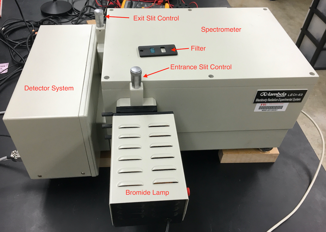
Fig. 5.1 Main parts of the black-body radiation experiment.

5.2.1. Spectrometer

The principle of the spectrometer is shown in Fig. 5.2. Light from the entrance slit is reflected and collimated by the mirror M1 and sent to a diffraction grating with 300 lines/mm. The diffracted and collimated light is then focused by mirror M2 onto the exit slit. In other word the image of the entrance slit is imaged to the exit slit at a wavelength that depends on the orientation of the diffraction grating.

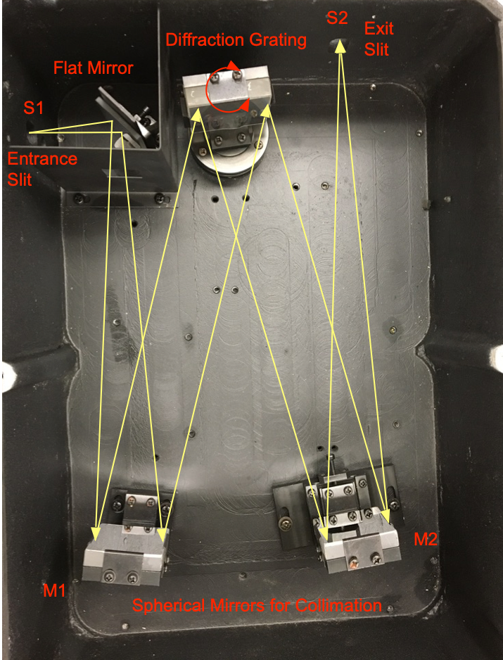
Fig. 5.2 Inside of the IR spectrometer with collimating mirrors, grating, entrance and exit slits. Two light rays are indicating the optic configuration and imaging properties of this instrument.

The exit slit in combination with the grating orientation selects the wavelength for which the intensity will be measured.

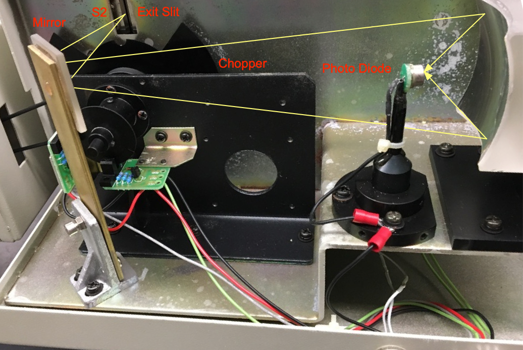
Fig. 5.3 The detector unit consisting of the chopper, the focusing mirror and the photo-sensor.

After the exit slit the light is focused on a photo-sensor to measure its intensity. The detector part also includes a chopper that makes it possible to integrate the photo-sensor signal over a defined time interval and helps with the suppression of background light (Fig. 5.3). The resulting signal is digitized and plotted as a function of wavelength by the control software (LEOI-63). Once a scan is completed you can save the measured data in a so-called ht file which can subsequently be read using the get_ht function included in the black-body software module.

5.3. Experimental Procedure

1. Turn on the IR spectrometer and then start the acquisition program LEOI-63 and initialize the spectrometer by clicking cancel on the pop-up dialog. If the dialoge does not appear you can do the initialization by using the menu item \({\rm Work} \rightarrow {\rm Initialize}\)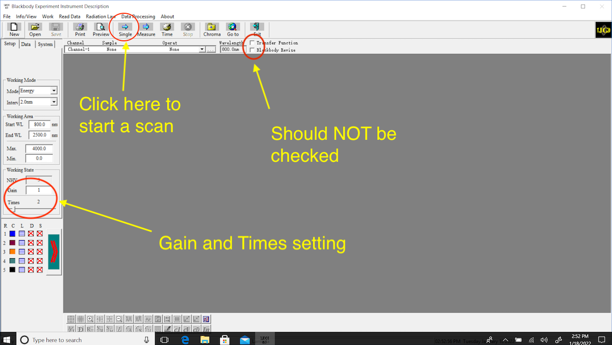

   

   Fig. 5.4 LEOI-63 startup screen with correct configuration.

2. Make sure that the check boxes Transfer function and Blackbody Revise are NOT checked. See (Fig. 5.4)

3. Make sure that the Gain is set to 1 and Times is set to 2 See (Fig. 5.4)

4. Set the lamp current to 2.5A and let the system warm-up for 15-20 minutes.

5. Set the entrance and exit slits to 0.45mm each. Make a scan by clicking on the toolbar item labeled Single (see Fig. 5.4) and make sure that the signal does not saturate the display (is less than 4000, see Fig. 5.5). Adjust the entrance slit width accordingly.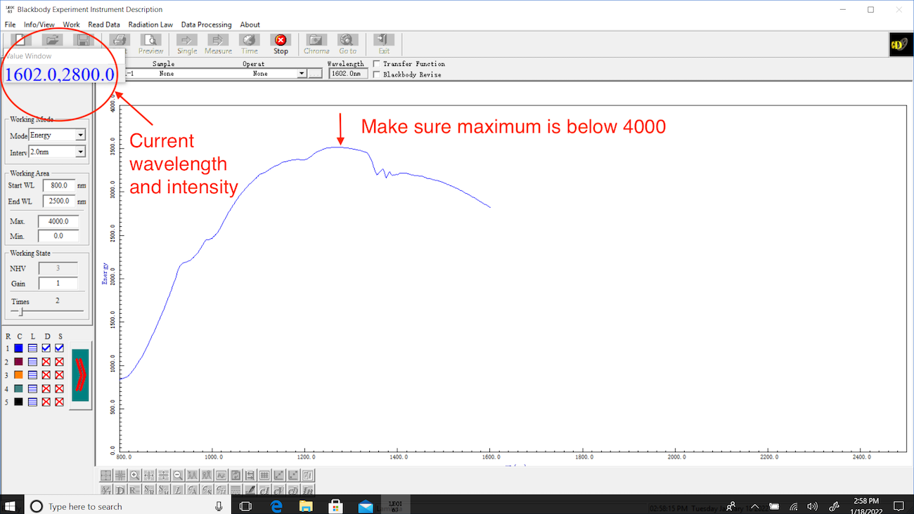

   

   Fig. 5.5 Performing a scan. The current wavelength and intensity are indicated in the top left corner.

6. Take a scan and save the resulting spectrum in a directory that you created for your group. This is your normalization spectrum

7. Take scans at 6 different lamp currents between the lowest and the highest current settings.

Once you are finished with your measurements set the grating to 800nm (click on the GoTo icon on the LEOI-63 toolbar and enter the wavelength in nm in the dialog window) and turn off the instrument and transfer your data to your computer.

5.4. Analysis

5.4.1. Overview

In the analysis of the data you will determine the instrument’s transfer function that is used to correct your raw data for variations in light detection efficiency due to different spectral responses of its optical elements and the light detector. In a second step the data are also corrected for variations in the responsivity of the photo sensor. After these corrections the measured spectrum should be proportional to a black body spectrum at a certain temperature. You will determine the temperature of the lamp filament by fitting a black body spectrum to your corrected spectrum using the temperature and an overall scaling factor as fit parameters. In order to be able to perform these tasks you can download the python module BB_analysis_tools which contains a function to calculate the tungsten emissivity, a function to correct the measured intensity for variations of the spectral responsivity of the photo-sensor and a function to load the saved data into python. Please follow the steps below to carry out the analysis and ask for help if and when you are stuck. You also need the data files W_emissivity.data, R_parameters.data and R_parameters_filter.data

The table below shows the color temperature of the Bromine-Tungsten lamp:

Current (A)	Color Temperature (K)
1.40	2150
1.50	2230
1.60	2330
1.70	2410
1.80	2490
1.90	2540
2.00	2610
2.10	2700
2.20	2770
2.30	2830
2.50	2940

Place the python module and data files into your analysis directory.

5.4.2. Analysis Steps

Follow the steps below to carry out your analysis. It is assumed that you have created a directory (folder) for this experiment and placed all your data files as well as the files described above there.

1. Create a new python script and import numpy and the LabTools box as ususal. Import the BB_analysis_tools by doing:

   import numpy as np
   import LT.box as B
   import BB_analysis_tools as BBT
   

2. Place the lamp data in a datafile and make a plot of lamp temperature as a function of lamp current and label the axes.

3. Fit a second order polynomial to lamp temperature as a function of current.

4. Load the normalization file (the first data set at a current setting of 2.50A) and store the wavelength and Intensities in arrays called e.g. lam_norm and I_norm. You can load your saved ht files as follows:

   l_exp, I_exp_raw = BBT.get_ht('my_file.ht')
   

   Here l_exp contains the wave lengths in nm and I_exp_raw the raw intensities

5. Make a plot of I_norm as a function of lam_norm to make sure the data look correct.

6. Initialize the emissivity calculation using the BB_analysis_tools:

   em = BBT.W_em()
   

7. Program the black body spectrum (5.6) as a Python function with the temperature and the wavelength as arguments and take care of the units used (your wavelengths are in nm). Call this function e.g. B_lt

8. Calculate the black-body spectrum for the normalization temperature \(T_{norm} = 2940K\) and your measured wavelengths lam_norm and store the result in a variable called I_calc.

9. Calculate the emissivity \(\epsilon(\lambda, T)\) for the given temperature and wavelengths using the function em as follows (note: this function expects the wavelengths in nm):

   em_norm = em(lam_norm, T_norm)
   

10. The product of your calculated emissivity and the calculated black-body spectrum is your expected intensity distribution for the bromine lamp at the normalization temperature (\(T_{norm}\)) and the experimental transfer function is now \(f_{tr} = \epsilon(\lambda, T) I_{calc}/I_{norm}\). Calculate this expression and store the result in the variable f_tr. All your measurement data need to be corrected by this as follows:

    I_exp_corr = I_exp_raw*f_tr  # I_exp are intensity data for any lamp temperature
    

11. Your transfer function corrected data need also be corrected for the wavelength dependent variation of the photo-sensor sensitivity (responsivity). Initialize the calculation using the photo_sensor class from the BB_analysis_tools:

    PD = BBT.photo_sensor('R_parameters.data', I_norm)   # I_norm has to be your uncorrected normalization spectrum
    

12. To calculate the sensitivity correction factors for a data set you use the member function (or attribute) corr of photo_sensor. As an example for loading a data set and calculate the corresponding correction factors

    l_exp, I_exp_raw = BBT.get_ht('exp_data_2.13.ht')    # measurement taken at a lamp current of 2.13 A
    p_corr = PD.corr(l_exp, I_exp_raw)                   # correction factors calculated for this measurement
    

13. To completely correct the the spectrum for transfer function and sensitivity you multiply the spectrum by the transfer function f_tr and the sensitivity correction factor p_corr and name this I_corr. This spectrum then corresponds to the actual spectrum of the lamp light at the entrance slit of the spectrometer.:

    I_corr = I_exp_raw*f_tr*p_corr
    

5.4.3. Data Fitting

1. The next step is to model the lamp spectrum and fit it to the measured and corrected spectrum for any lamp current. This allows one to determine the temperature of the lamp filament (and e.g. check the provided lamp data). The model spectrum for the Bromine lamp is based on (5.8) i.e. the product of the emissivity, a black-body spectrum and an overall factor.

2. Setup two fit parameters, one for the temperature called T_f and one for a scale factor called A. Initialize T_f with 2000 and A with 1.

3. Write a fit function called I_fit that takes the wavelength as an argument and calculated the product of equation (5.8) with these fit parameters and returns the calculated intensity.

4. Fit your corrected spectra, make a plot of the data and the fit and store the fit parameters in a list.

5. Compare your fitted temperatures to the value you get from the polynomial fitted to the lamp data. How well do they agree or disagree?

6. Using your fitted temperatures and the scale factors correct your experimental intensities I_corr for the calculated emissivity and the fitted scale factor by dividing I_corr by these two quantities. This gives you an experimental version of a Black-Body spectrum and call it BB_exp

7. Wien’s law states that the product of the wavelength of the maximum of the intensity distribution for a black body and its temperature is a constant. Form your BB_exp data determine the location of their maxima. Make a plot of the product of the fitted temperatures to the wavelengths of the maxima as a function of temperature. Compare this value to the predicted one. Estimate the uncertainty of this product.

8. Make a plot of the logarithm of the integrated experimental black-body spectra (BB_exp) as a function of the logarithm of the fitted temperatures and fit a line to these data. According to the Stefan-Boltzmann law the slope of this line should be 4. (see (5.7) and the analysis hint below)

9. Since only wavelengths between 800 nm and 250 nm were measured, the integral over the experimental black-body spectra is incomplete. Using the fitted spectra calculate the contributions between 1 nm and 800 nm and between 2500 nm and 10000 nm and add them to the experimental values. Fit the corrected data and compare the two slopes. What did you find?

5.4.4. Analysis Hints: Numerical Integration

You have an array for the experimental Black-Body spectrum (BB_exp) and the corresponding wavelengths l_exp or l_norm. A simple approximation of the integral of BB_exp between l_min and l_max is to calculate the corresponding Riemann sum

sel = B.in_between(l_min, l_max, l_exp)  # find which wavelengths values are between l_min and l_max
dl = l_exp[1] - l_exp[0]                 # this corresponds to dlambda
S = np.sum(BB_exp[sel])*dl               # this would be the intergral of BB_exp dlambda from l_min to l_max

A better approximation is available from numpy using the the composite trapezoidal rule. In this case you would do

sel = B.in_between(l_min, l_max, l_exp)  # find which wavelengths values are between l_min and l_max
S = np.trapz(BB_exp[sel], x = l_exp[sel])

This would be a better approximation.